02: Getting Started with a Simple Request

Dr. Nelson Roque

Goals of this Notebook

This notebook demonstrates how to download and stack EPA AirData files for 1991-1992 focusing on Ozone (44201) data.

---

The simplest request retrieves EPA AirData for a specific analyte (pollutant) over a given time range (e.g., download daily ozone (44201) data for 1991-1992).

library(tidypollute)
ozone <- get_epa_airdata(analyte = "44201", start_year = 1991, end_year = 1992, freq = "daily")

## 
## Preparing to download:
## Analyte: 44201 
## Years: 1991 to 1992 
## Number of files: 2 
## Freq of data: daily 
## Output directory: data/

# Load necessary libraries
library(tidyverse)
library(ggplot2)
library(patchwork)
library(viridis)
library(hrbrthemes)
library(extrafont)
library(lubridate)  # For handling dates

# Ensure Helvetica or Arial is available
loadfonts(device = "win")
theme_set(theme_minimal(base_family = "Helvetica"))  # Use Arial if Helvetica isn't available

# ---- Data Preparation ----

# Convert date_local to Date format
ozone_f <- ozone %>%
  mutate(date_local = as.Date(date_local),
         day_of_week = wday(date_local, label = TRUE, abbr = FALSE),
         week_of_year = isoweek(date_local),
         year = year(date_local)) %>%
  filter(year == 1992) %>%
  full_join(us_states) %>%
  mutate(max_hour = as.numeric(x1st_max_hour))

# Aggregate mean ozone levels per day
ozone_summary <- ozone_f %>%
  group_by(date_local, state_region) %>%
  summarise(mean_ozone = mean(arithmetic_mean, na.rm = TRUE))

# Define key holidays
holidays <- tibble(
  date_local = as.Date(c("1991-07-04", "1991-12-01", "1992-07-04", "1992-12-01")),
  holiday = c("July 4", "Dec 1", "July 4", "Dec 1")
)

# ---- Panel 1: Heatmap ----

heatmap_plot <- ggplot(ozone_f, aes(x = date_local, y = max_hour, fill = x1st_max_value)) +
  geom_tile() +
  scale_fill_viridis(option = "magma", name = "Ozone Level", direction = -1) +
  labs(
    title = "Hour of Worst (Max) Ozone Concentrations",
    x = "Date",
    y = "Hour of Day"
  ) +
  theme_minimal(base_family = "Helvetica") +
  theme(
    plot.title = element_text(size = 18, face = "bold", margin = margin(b = 10)),
    axis.title = element_text(size = 14, face = "bold"),
    axis.text = element_text(size = 12),
    legend.position = "right"
  )
heatmap_plot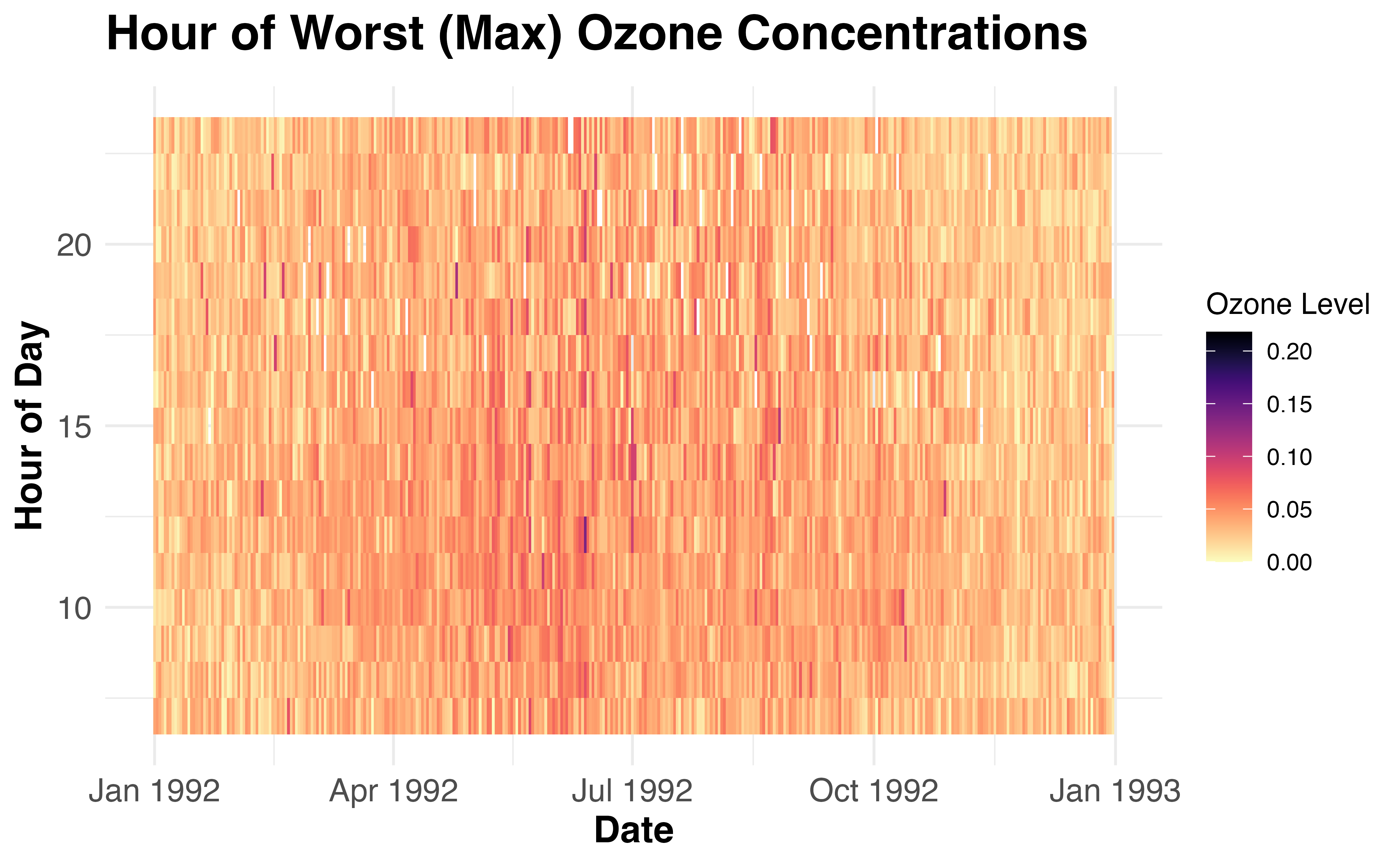

# ---- Panel 2: Time Series with WHO Thresholds ----
time_series_plot <- ggplot(ozone_summary, aes(x = date_local, y = mean_ozone)) +
  #geom_line(color = "#0072B2", size = 1.2, alpha = 0.8) +
  geom_jitter(color = "#D55E00", size = 2, alpha = 0.4) +
  # geom_hline(data = who_thresholds, aes(yintercept = threshold, linetype = label), color = "gray50") +
  geom_vline(data = holidays, aes(xintercept = as.numeric(date_local)), linetype = "dashed", color = "red", size = 0.8) +
  labs(
    title = "Daily Average Ozone Levels",
    x = "Date",
    y = "Ozone (ppm)"
  ) +
  theme_minimal(base_family = "Helvetica") +
  theme(
    plot.title = element_text(size = 18, face = "bold", margin = margin(b = 10)),
    axis.title = element_text(size = 14, face = "bold"),
    axis.text = element_text(size = 10),
    plot.caption = element_text(size = 10, face = "italic", hjust = 1),
    legend.position = "bottom"
  ) +
  facet_grid(.~ state_region)

time_series_plot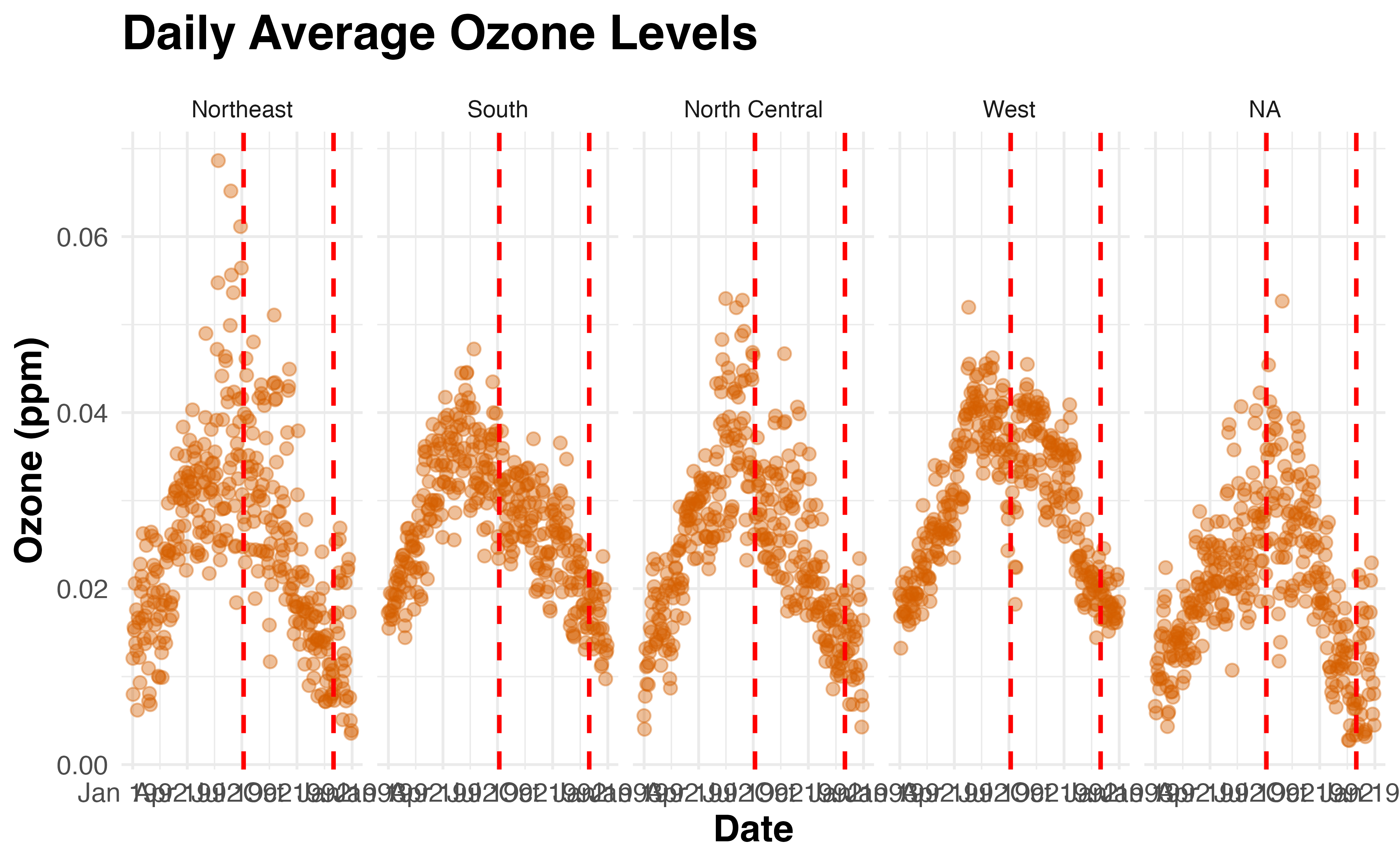

# ---- Panel 3: Variability by Week & Day of the Week ----

variability_plot <- ggplot(ozone_f, aes(x = week_of_year, y = arithmetic_mean, group = week_of_year)) +
  geom_boxplot(fill = "#0072B2", alpha = 0.5) +
  facet_wrap(~ day_of_week, scales = "free_y") +
  labs(
    title = "Ozone Variability by Week & Day",
    x = "Week of Year",
    y = "Ozone (ppm)"
  ) +
  theme_minimal(base_family = "Helvetica") +
  theme(
    plot.title = element_text(size = 18, face = "bold", margin = margin(b = 10)),
    axis.title = element_text(size = 14, face = "bold"),
    axis.text = element_text(size = 12),
    strip.text = element_text(size = 12, face = "bold")
  )

variability_plot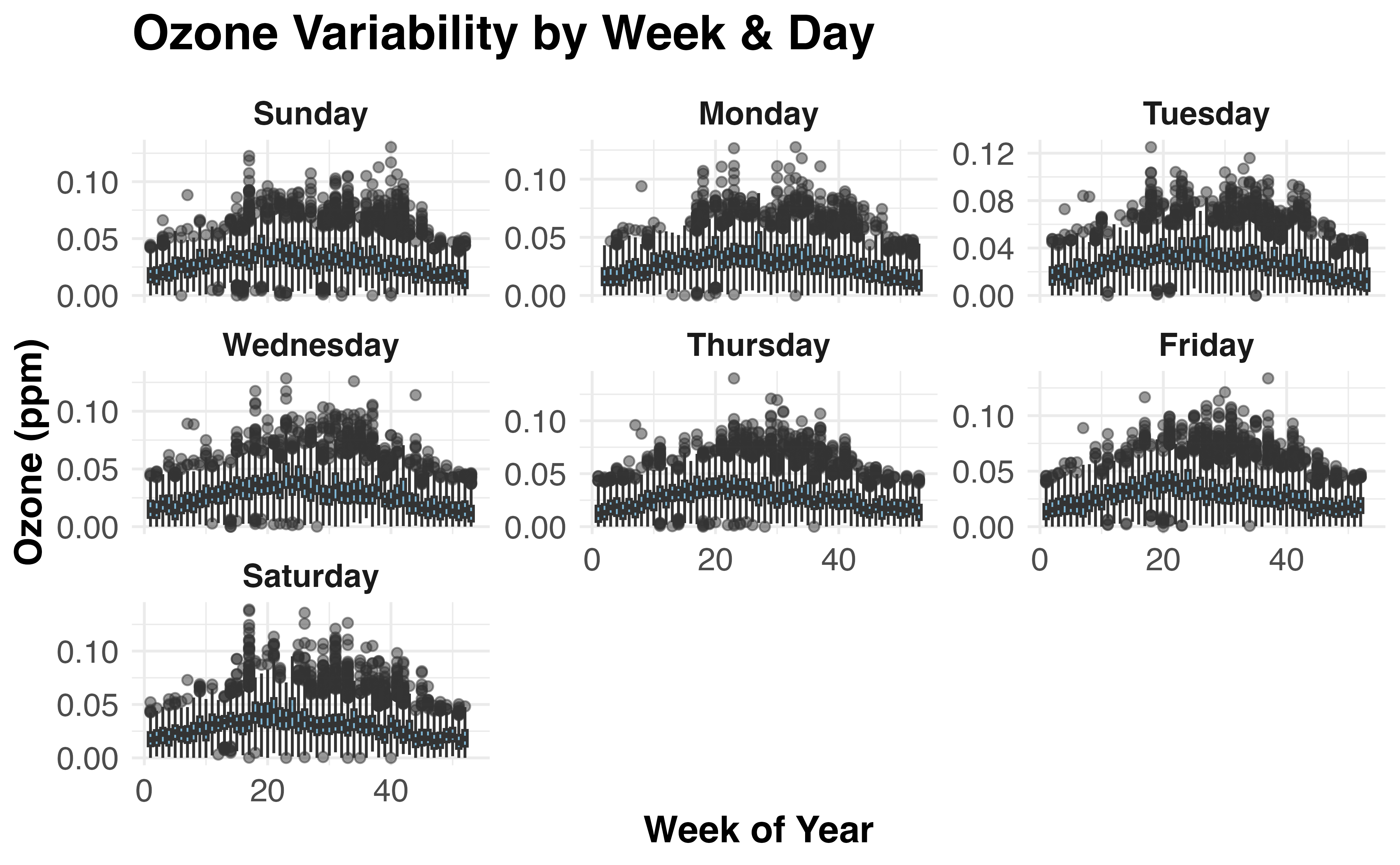

# ---- Combine Plots Using Patchwork ----

final_plot <- (heatmap_plot / time_series_plot / variability_plot) +
  plot_annotation(
    title = "Ozone Levels Over Time",
    subtitle = "Hourly Concentrations, Daily Trends with WHO Guidelines, and Weekly Variability",
    caption = "Data Source: EPA AirData (https://aqs.epa.gov/aqsweb/airdata/download_files.html)",
    theme = theme(
      plot.title = element_text(size = 22, face = "bold", margin = margin(b = 12)),
      plot.subtitle = element_text(size = 16, margin = margin(b = 8)),
      plot.caption = element_text(size = 12, face = "italic", hjust = 1)
    )
  )

---

Summary

This notebook provides a simple workflow for retrieving EPA AirData using tidypollute.

You can:

✅ Retrieve and filter dataset links (to zip files).
✅ Download specific pollutant data (e.g., Ozone, Wind).
✅ Stack and process the downloaded files.
✅ Scales up to download all available EPA AirData.

For more details, check out tidypollute documentation.