Ch. 8 Data Wrangling and Visualization of Big Data
8.1 Overview
For this example, we are working with the Google Community Mobility Reports dataset.
“These Community Mobility Reports aim to provide insights into what has changed in response to policies aimed at combating COVID-19. The reports chart movement trends over time by geography, across different categories of places such as retail and recreation, groceries and pharmacies, parks, transit stations, workplaces, and residential.”
8.3 Read in data
# read in the Google Mobility dataset
google_mobility <- read_csv("https://www.gstatic.com/covid19/mobility/Global_Mobility_Report.csv")
## Rows: 10392488 Columns: 15
## ── Column specification ─────────────────────────────────────────────────────────────────
## Delimiter: ","
## chr (8): country_region_code, country_region, sub_region_1, sub_region_2, m...
## dbl (6): retail_and_recreation_percent_change_from_baseline, grocery_and_ph...
## date (1): date
##
## ℹ Use `spec()` to retrieve the full column specification for this data.
## ℹ Specify the column types or set `show_col_types = FALSE` to quiet this message.8.5 Create lookup tables
R, as well as some packages, have built in datasets. They can be called with the data() function (e.g., data(state)). We will leverage a built in dataset with state metadata.
data(state)
state_lookup = tibble(sub_region_1 = state.name,
                      us_division = state.division,
                      us_region = state.region,
                      state_land_area = state.area)

# for more state data, look at the following data object (data from 1970s)
state.x77
## Population Income Illiteracy Life Exp Murder HS Grad Frost
## Alabama 3615 3624 2.1 69.05 15.1 41.3 20
## Alaska 365 6315 1.5 69.31 11.3 66.7 152
## Arizona 2212 4530 1.8 70.55 7.8 58.1 15
## Arkansas 2110 3378 1.9 70.66 10.1 39.9 65
## California 21198 5114 1.1 71.71 10.3 62.6 20
## Colorado 2541 4884 0.7 72.06 6.8 63.9 166
## Connecticut 3100 5348 1.1 72.48 3.1 56.0 139
## Delaware 579 4809 0.9 70.06 6.2 54.6 103
## Florida 8277 4815 1.3 70.66 10.7 52.6 11
## Georgia 4931 4091 2.0 68.54 13.9 40.6 60
## Hawaii 868 4963 1.9 73.60 6.2 61.9 0
## Idaho 813 4119 0.6 71.87 5.3 59.5 126
## Illinois 11197 5107 0.9 70.14 10.3 52.6 127
## Indiana 5313 4458 0.7 70.88 7.1 52.9 122
## Iowa 2861 4628 0.5 72.56 2.3 59.0 140
## Kansas 2280 4669 0.6 72.58 4.5 59.9 114
## Kentucky 3387 3712 1.6 70.10 10.6 38.5 95
## Louisiana 3806 3545 2.8 68.76 13.2 42.2 12
## Maine 1058 3694 0.7 70.39 2.7 54.7 161
## Maryland 4122 5299 0.9 70.22 8.5 52.3 101
## Massachusetts 5814 4755 1.1 71.83 3.3 58.5 103
## Michigan 9111 4751 0.9 70.63 11.1 52.8 125
## Minnesota 3921 4675 0.6 72.96 2.3 57.6 160
## Mississippi 2341 3098 2.4 68.09 12.5 41.0 50
## Missouri 4767 4254 0.8 70.69 9.3 48.8 108
## Montana 746 4347 0.6 70.56 5.0 59.2 155
## Nebraska 1544 4508 0.6 72.60 2.9 59.3 139
## Nevada 590 5149 0.5 69.03 11.5 65.2 188
## New Hampshire 812 4281 0.7 71.23 3.3 57.6 174
## New Jersey 7333 5237 1.1 70.93 5.2 52.5 115
## New Mexico 1144 3601 2.2 70.32 9.7 55.2 120
## New York 18076 4903 1.4 70.55 10.9 52.7 82
## North Carolina 5441 3875 1.8 69.21 11.1 38.5 80
## North Dakota 637 5087 0.8 72.78 1.4 50.3 186
## Ohio 10735 4561 0.8 70.82 7.4 53.2 124
## Oklahoma 2715 3983 1.1 71.42 6.4 51.6 82
## Oregon 2284 4660 0.6 72.13 4.2 60.0 44
## Pennsylvania 11860 4449 1.0 70.43 6.1 50.2 126
## Rhode Island 931 4558 1.3 71.90 2.4 46.4 127
## South Carolina 2816 3635 2.3 67.96 11.6 37.8 65
## South Dakota 681 4167 0.5 72.08 1.7 53.3 172
## Tennessee 4173 3821 1.7 70.11 11.0 41.8 70
## Texas 12237 4188 2.2 70.90 12.2 47.4 35
## Utah 1203 4022 0.6 72.90 4.5 67.3 137
## Vermont 472 3907 0.6 71.64 5.5 57.1 168
## Virginia 4981 4701 1.4 70.08 9.5 47.8 85
## Washington 3559 4864 0.6 71.72 4.3 63.5 32
## West Virginia 1799 3617 1.4 69.48 6.7 41.6 100
## Wisconsin 4589 4468 0.7 72.48 3.0 54.5 149
## Wyoming 376 4566 0.6 70.29 6.9 62.9 173
## Area
## Alabama 50708
## Alaska 566432
## Arizona 113417
## Arkansas 51945
## California 156361
## Colorado 103766
## Connecticut 4862
## Delaware 1982
## Florida 54090
## Georgia 58073
## Hawaii 6425
## Idaho 82677
## Illinois 55748
## Indiana 36097
## Iowa 55941
## Kansas 81787
## Kentucky 39650
## Louisiana 44930
## Maine 30920
## Maryland 9891
## Massachusetts 7826
## Michigan 56817
## Minnesota 79289
## Mississippi 47296
## Missouri 68995
## Montana 145587
## Nebraska 76483
## Nevada 109889
## New Hampshire 9027
## New Jersey 7521
## New Mexico 121412
## New York 47831
## North Carolina 48798
## North Dakota 69273
## Ohio 40975
## Oklahoma 68782
## Oregon 96184
## Pennsylvania 44966
## Rhode Island 1049
## South Carolina 30225
## South Dakota 75955
## Tennessee 41328
## Texas 262134
## Utah 82096
## Vermont 9267
## Virginia 39780
## Washington 66570
## West Virginia 24070
## Wisconsin 54464
## Wyoming 972038.6 Pre-process data
- filter data
- add meta-date features (month, year, day, etc)
# >>>>>>>>>>>>>>>>>>>>>>>>>>>>>>>>>>>>>>>>>>>>>>>>>>>>>>>>>>>>>>>>>>>>>>>>>>>>>>

# filter for US
google_mobility_US <- google_mobility %>%
  filter(country_region == "United States") %>%
  mutate(dt_date = date) %>%
  mutate(dt_month = lubridate::month(dt_date),
         dt_month_ = lubridate::month(dt_date, label=T),
         dt_year= lubridate::year(dt_date),
         dt_day = lubridate::day(dt_date),
         dt_wkday_l = lubridate::wday(dt_date, label=T),
         dt_wkday_n = lubridate::wday(dt_date)) %>%
  mutate(dt_weekend = ifelse(dt_wkday_l %in% c("Sat", "Sun"), TRUE, FALSE))
8.7 Joining datasets
- Merge Google Mobility dataset with R data for US states
google_mobility_US_w_lu <- google_mobility_US %>%
  inner_join(state_lookup)
## Joining, by = "sub_region_1"8.8 Quick descriptives
- single line of code descriptives across a dataset
#skimr::skim(google_mobility_US)8.9 Filter data
- filter with specific entries
- filter for a collection of entries
# filter with specific entries
google_mobility_US_NY <- google_mobility_US %>%
  filter(sub_region_1 == "New York")

google_mobility_US_FL <- google_mobility_US %>%
  filter(sub_region_1 == "Florida")

# >>>>>>>>>>>>>>>>>>>>>>>>>>>>>>>>>>>>>>>>>>>>>>>>>>>>>>>>>>>>>>>>>>>>>>>>>>>>>>

# filter to a 'vector' of entries
google_mobility_US_targeted <- google_mobility_US %>%
  filter(sub_region_1 %in% c("California", "New York", "Florida"))
8.10 Compute aggregates
# base R approach
table(google_mobility_US$sub_region_1)
##
## Alabama Alaska Arizona
## 54866 8699 13531
## Arkansas California Colorado
## 53846 48318 38559
## Connecticut Delaware District of Columbia
## 7767 3452 863
## Florida Georgia Hawaii
## 56781 116246 4315
## Idaho Illinois Indiana
## 28010 76376 76459
## Iowa Kansas Kentucky
## 71643 46353 80123
## Louisiana Maine Maryland
## 49323 14345 21416
## Massachusetts Michigan Minnesota
## 12505 65941 63831
## Mississippi Missouri Montana
## 58235 80247 22623
## Nebraska Nevada New Hampshire
## 38138 10732 9468
## New Jersey New Mexico New York
## 18978 24916 53244
## North Carolina North Dakota Ohio
## 82033 16312 75182
## Oklahoma Oregon Pennsylvania
## 53005 28646 56170
## Rhode Island South Carolina South Dakota
## 5169 39446 21719
## Tennessee Texas Utah
## 74908 163937 19814
## Vermont Virginia Washington
## 11754 103423 30440
## West Virginia Wisconsin Wyoming
## 36130 57815 16418
# number of records by state
records_per_state = google_mobility_US %>%
  group_by(sub_region_1) %>%
  summarise(n_records = n()) %>%
  arrange(sub_region_1)
records_per_state
## # A tibble: 52 × 2
## sub_region_1 n_records
## <chr> <int>
## 1 Alabama 54866
## 2 Alaska 8699
## 3 Arizona 13531
## 4 Arkansas 53846
## 5 California 48318
## 6 Colorado 38559
## 7 Connecticut 7767
## 8 Delaware 3452
## 9 District of Columbia 863
## 10 Florida 56781
## # … with 42 more rows
# >>>>>>>>>>>>>>>>>>>>>>>>>>>>>>>>>>>>>>>>>>>>>>>>>>>>>>>>>>>>>>>>>>>>>>>>>>>>>>

# group data by weekday
metrics_month_weekend_US <- google_mobility_US %>%
  group_by(sub_region_1, dt_year, dt_month_, dt_wkday_l) %>%
  summarise(avg_change_parks = mean(parks_percent_change_from_baseline, na.rm=T),
            avg_change_retail_rec = mean(retail_and_recreation_percent_change_from_baseline, na.rm=T),
            avg_change_workplaces = mean(workplaces_percent_change_from_baseline, na.rm=T)) %>%
  inner_join(state_lookup)
## `summarise()` has grouped output by 'sub_region_1', 'dt_year', 'dt_month_'. You can
## override using the `.groups` argument.
## Joining, by = "sub_region_1"8.11 Visualize the data
# plot summary data across all states
allUS_retail = ggplot(metrics_month_weekend_US %>% filter(us_region %in% c("South", "West")), aes(sub_region_1, avg_change_retail_rec)) +
  geom_boxplot() +
  theme_minimal() +
  theme(axis.text.x=element_text(angle=90)) +
  facet_wrap(dt_year~.) +
  labs(x="Month", y="Retail (% Change)")

allUS_parks = ggplot(metrics_month_weekend_US %>% filter(us_region %in% c("South", "West")), aes(sub_region_1, avg_change_parks)) +
  geom_boxplot() +
  theme_minimal() +
  facet_wrap(dt_year~.) +
  theme(axis.text.x=element_text(angle=90)) +
  labs(x="Month", y="Parks (% Change)")

allUS_retail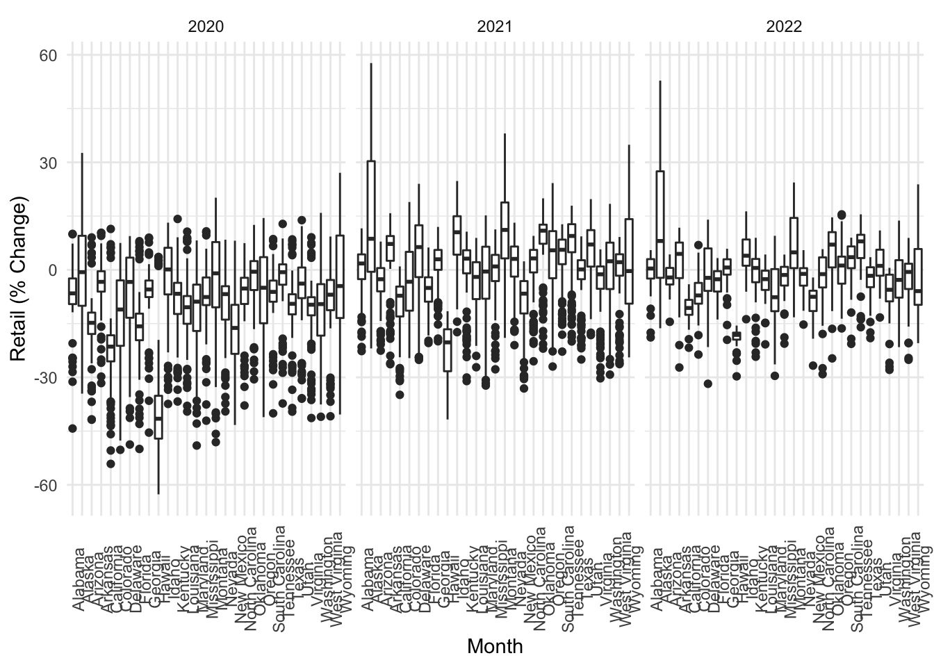
allUS_parks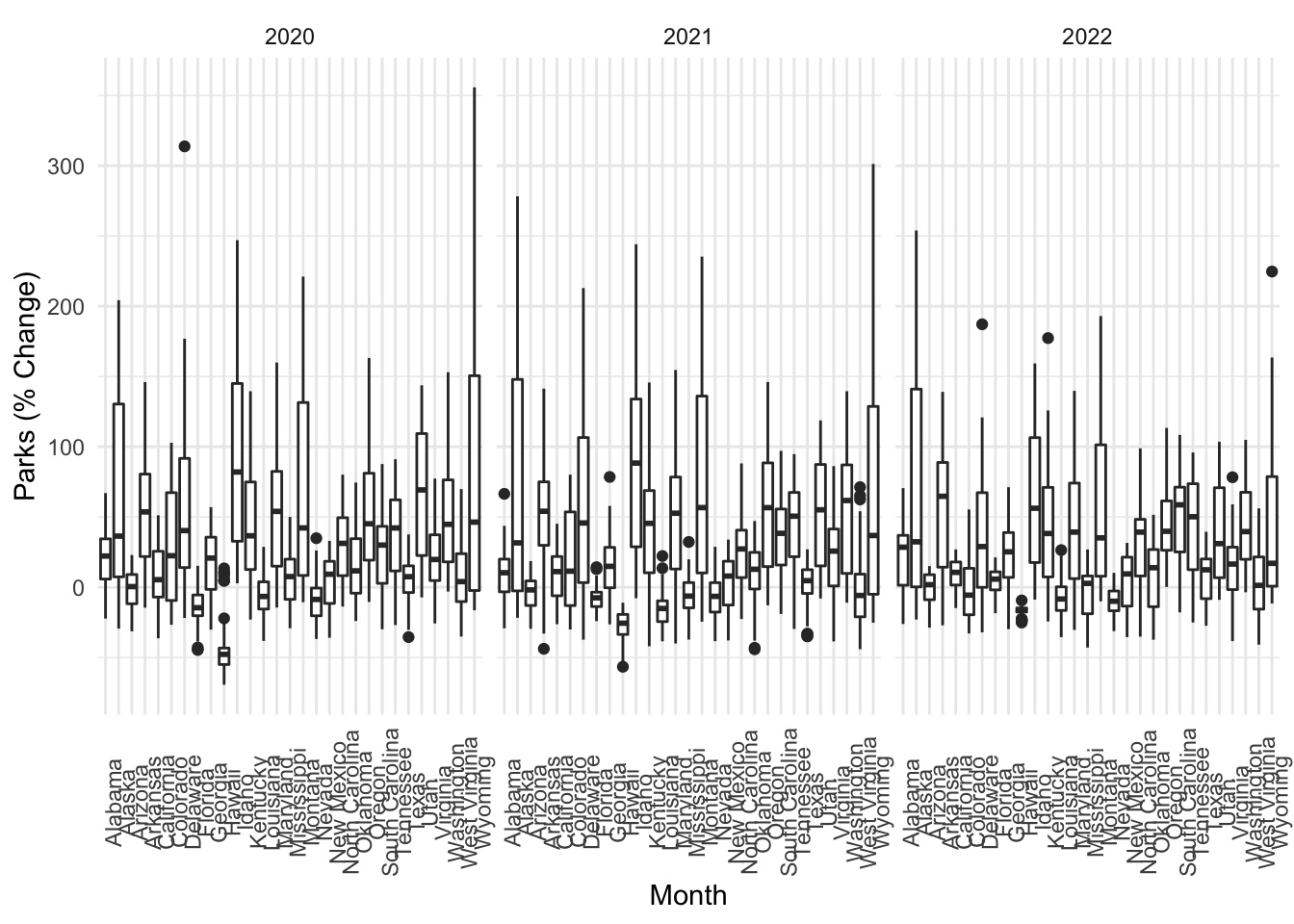
jitter_retail <- ggplot(metrics_month_weekend_US, aes(dt_month_,
                                     avg_change_retail_rec,
                                     group=us_region,
                                     color=us_region)) +
  #geom_point() +
  geom_jitter() +
  theme_minimal() +
  labs(x="Month", y="Retail & Recreation (% Change)")

smooth_retail = ggplot(metrics_month_weekend_US, aes(dt_month_,
                                     avg_change_retail_rec,
                                     group=us_region,
                                     color=us_region)) +
  #geom_point() +
  #geom_jitter() +
  geom_smooth() +
  theme_minimal() +
  labs(x="Month", y="Retail & Recreation (% Change)")

smooth_parks = ggplot(metrics_month_weekend_US, aes(dt_month_,
                                     avg_change_parks,
                                     group=us_region,
                                     color=us_region)) +
  #geom_point() +
  #geom_jitter() +
  geom_smooth() +
  theme_minimal() +
  labs(x="Month", y="Parks (% Change)")

jitter_retail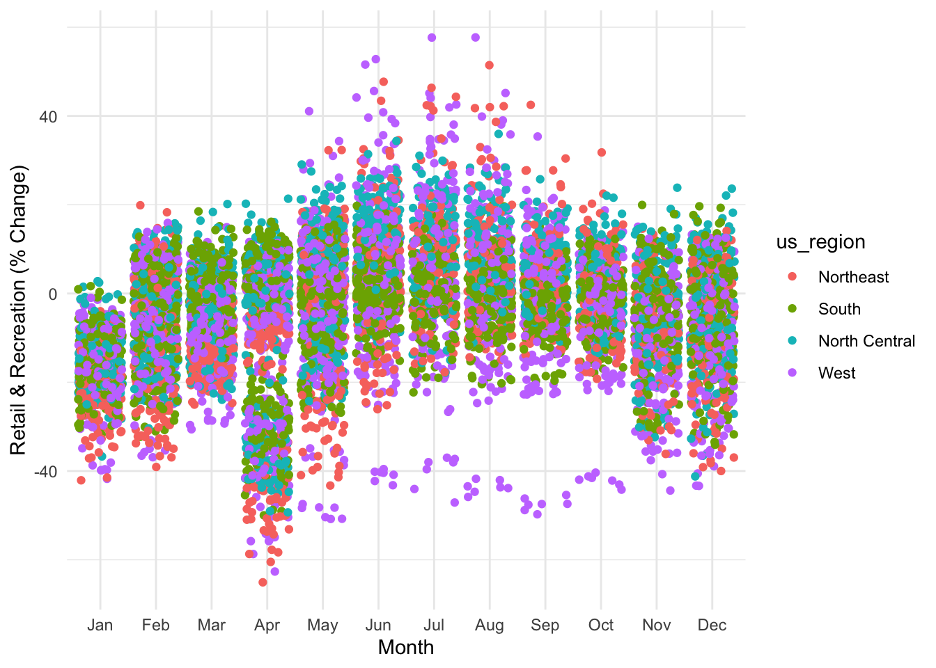
smooth_retail## `geom_smooth()` using method = 'gam' and formula 'y ~ s(x, bs = "cs")'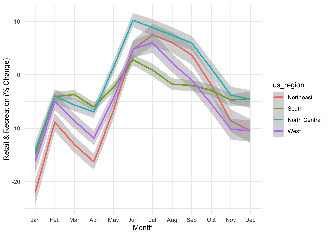
smooth_parks## `geom_smooth()` using method = 'gam' and formula 'y ~ s(x, bs = "cs")'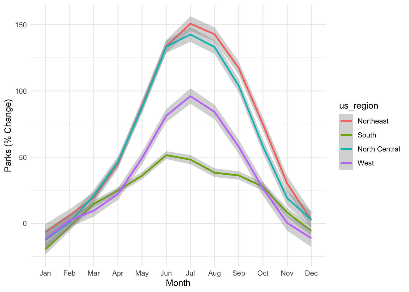
8.12 Combining multiple plots
library(cowplot)

# create a plot of weekly trends
early_covid_retail = ggplot(google_mobility_US_targeted %>%
         filter(dt_month %in% c(1,2,3,4,5)) %>%
         filter(dt_year == 2020), aes(dt_date,
                                    retail_and_recreation_percent_change_from_baseline,
                                    color=sub_region_1)) +
  #geom_point() +
  geom_jitter() +
  theme_minimal() +
  facet_wrap(.~sub_region_1) +
  labs(x="Month", y="Retal & Rec (% Change)", title="2020")

early_covid_parks = ggplot(google_mobility_US_targeted %>%
         filter(dt_month %in% c(1,2,3,4,5)) %>%
         filter(dt_year == 2020), aes(dt_date,
                                    parks_percent_change_from_baseline,
                                    color=sub_region_1)) +
  #geom_point() +
  geom_jitter() +
  theme_minimal() +
  facet_wrap(.~sub_region_1) +
  labs(x="Month", y="Parks (% Change)", title="2020")

nxtyear_covid_retail = ggplot(google_mobility_US_targeted %>%
         filter(dt_month %in% c(1,2,3,4,5)) %>%
         filter(dt_year == 2021), aes(dt_date,
                                    retail_and_recreation_percent_change_from_baseline,
                                    color=sub_region_1)) +
  #geom_point() +
  geom_jitter() +
  theme_minimal() +
  facet_wrap(.~sub_region_1) +
  labs(x="Month", y="Retal & Rec (% Change)", title="2021")
cowplot::plot_grid(early_covid_retail, early_covid_parks, ncol=1)## Warning: Removed 2050 rows containing missing values (geom_point).## Warning: Removed 7320 rows containing missing values (geom_point).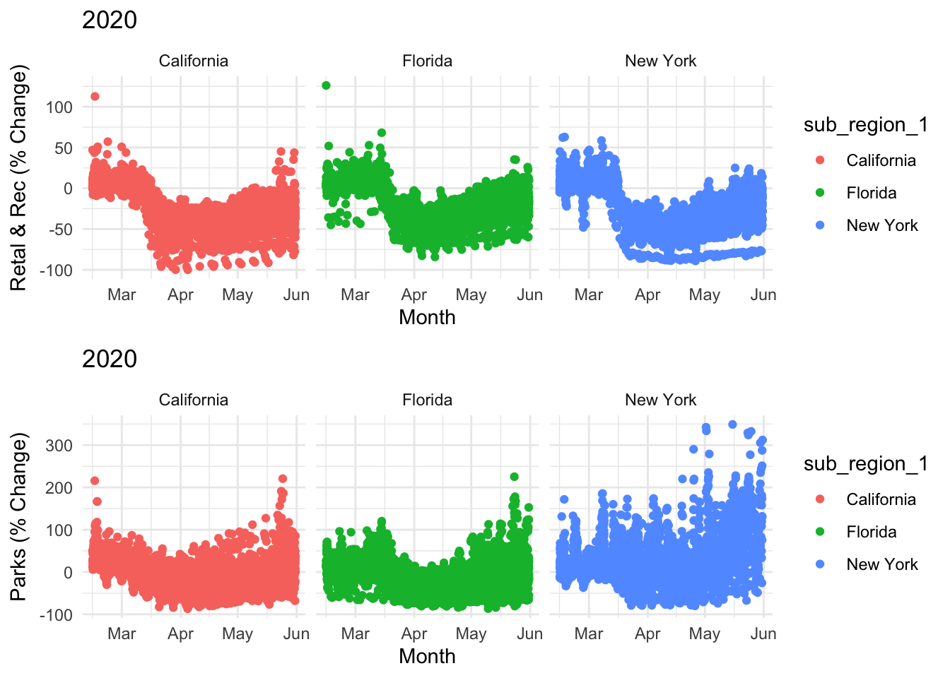
cowplot::plot_grid(early_covid_retail, nxtyear_covid_retail, ncol=1)## Warning: Removed 2050 rows containing missing values (geom_point).## Warning: Removed 2915 rows containing missing values (geom_point).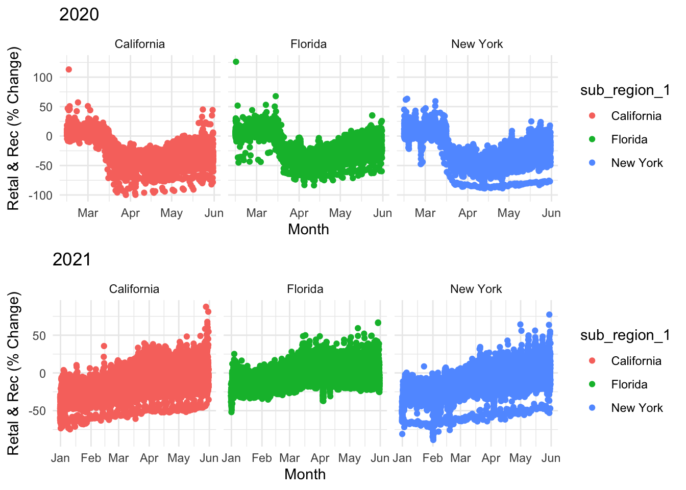
cowplot::plot_grid(allUS_retail, allUS_parks, ncol=1)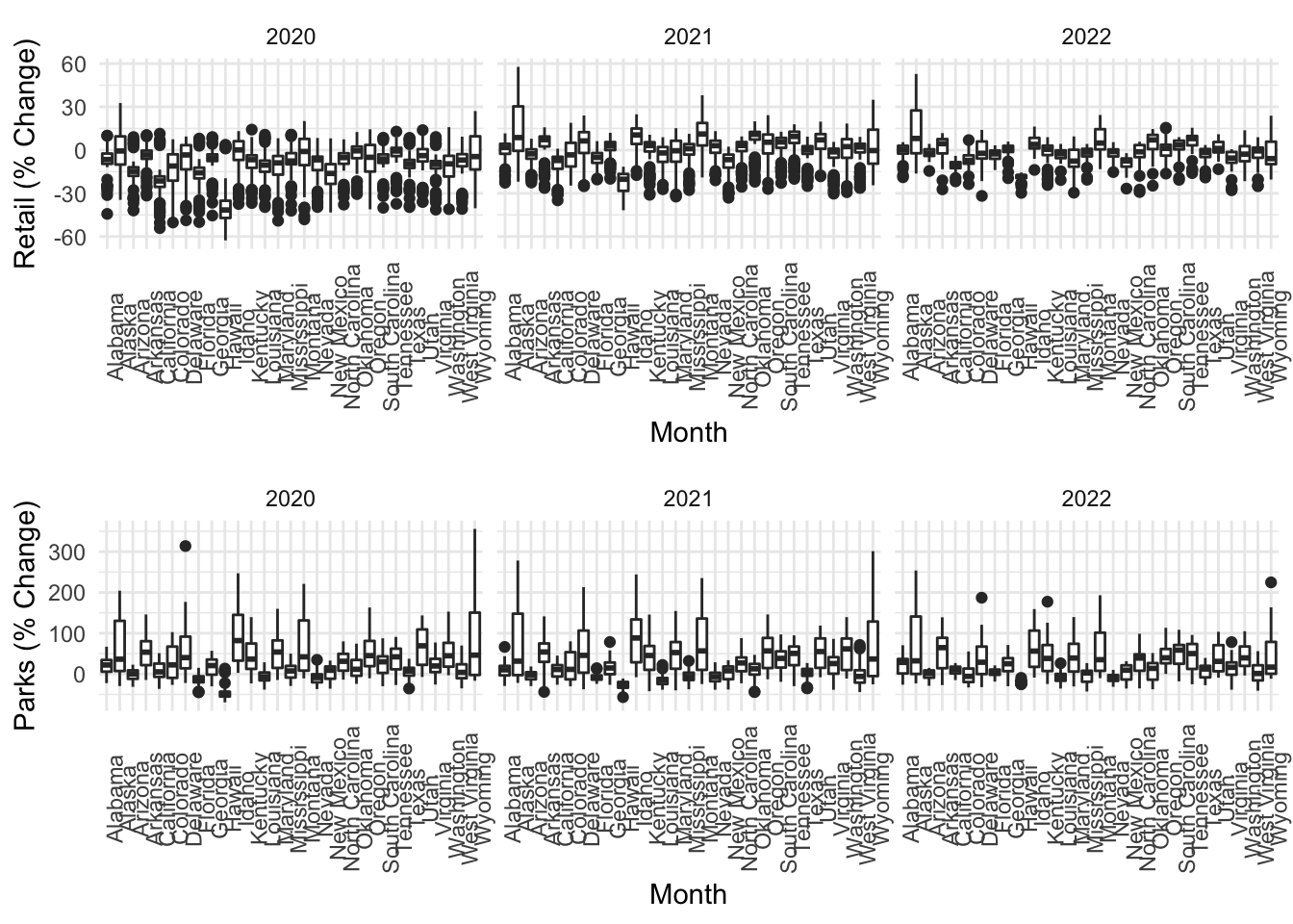
cowplot::plot_grid(smooth_retail, smooth_parks, ncol=1)## `geom_smooth()` using method = 'gam' and formula 'y ~ s(x, bs = "cs")'
## `geom_smooth()` using method = 'gam' and formula 'y ~ s(x, bs = "cs")'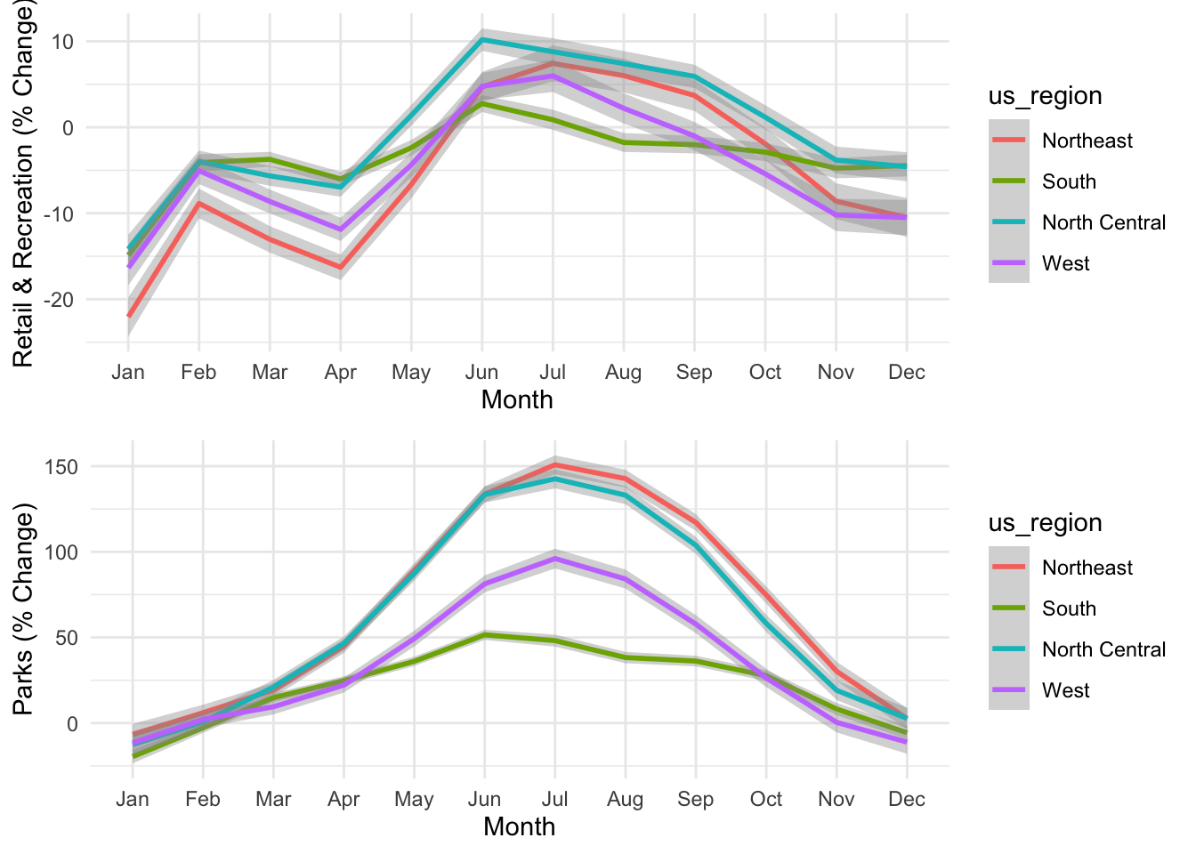
8.13 Filter dataset for next plots
# Variable names -----
#   retail_and_recreation_percent_change_from_baseline = col_double(),
#   grocery_and_pharmacy_percent_change_from_baseline = col_double(),
#   parks_percent_change_from_baseline = col_double(),
#   transit_stations_percent_change_from_baseline = col_double(),
#   workplaces_percent_change_from_baseline = col_double(),
#   residential_percent_change_from_baseline = col_double()


early_covid_period_data = google_mobility_US_w_lu %>%
         filter(dt_month %in% c(1,2,3,4,5,6)) %>%
         filter(dt_year == 2020) %>%
         filter(sub_region_1 %in% c("New York", "California", "Florida", "Wyoming", "Texas", "Arizona","Montana", "South Dakota", "Nevada"))
8.14 Styling your plots (theme_*)
ggplot(early_covid_period_data, aes(dt_date,
                                    parks_percent_change_from_baseline,
                                    color=sub_region_1)) +
  #geom_point() +
  theme_void() +
  geom_jitter() +
  facet_wrap(.~sub_region_1) +
  theme(legend.position = "none")
## Warning: Removed 40493 rows containing missing values (geom_point).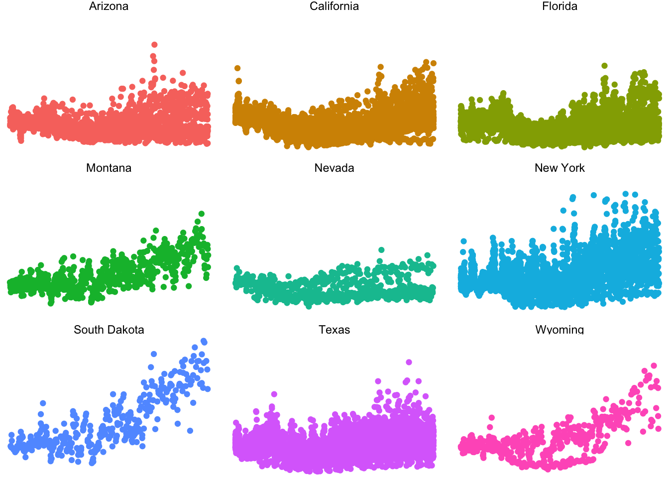
ggplot(early_covid_period_data, aes(dt_date,
                                    parks_percent_change_from_baseline,
                                    color=sub_region_1)) +
  geom_jitter() +
  facet_wrap(.~sub_region_1)
## Warning: Removed 40493 rows containing missing values (geom_point).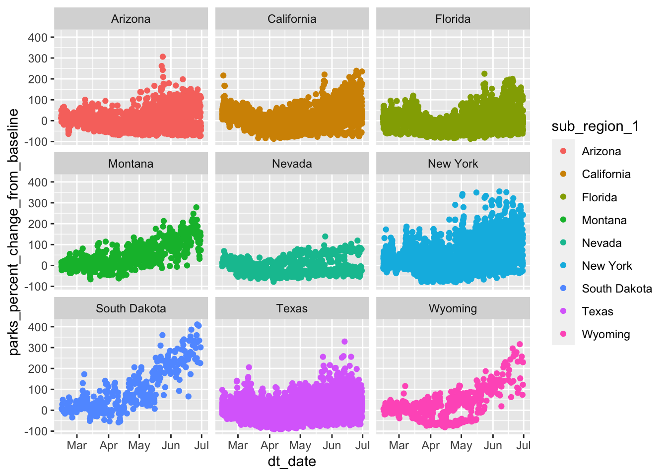
ggplot(early_covid_period_data, aes(dt_date,
                                    parks_percent_change_from_baseline,
                                    color=sub_region_1)) +
  #geom_point() +
  theme_bw() +
  geom_jitter() +
  facet_wrap(.~sub_region_1)
## Warning: Removed 40493 rows containing missing values (geom_point).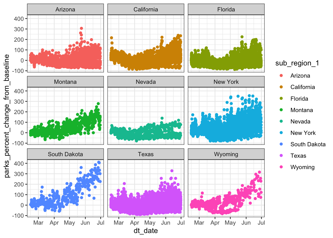
ggplot(early_covid_period_data, aes(dt_date,
                                    parks_percent_change_from_baseline,
                                    color=sub_region_1)) +
  #geom_point() +
  theme_dark() +
  geom_jitter() +
  facet_wrap(.~sub_region_1)
## Warning: Removed 40493 rows containing missing values (geom_point).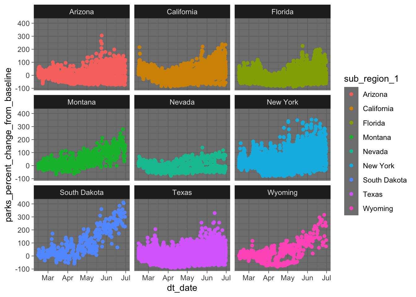
8.15 Production plots
ggplot(early_covid_period_data, aes(dt_date,
                                    parks_percent_change_from_baseline,
                                    color=us_region)) +
  #geom_point() +
  theme_bw() +
  geom_jitter() +
  facet_wrap(.~sub_region_1) +
  labs(x= "Date", y="Retail & Recreation (% Change)")
## Warning: Removed 40493 rows containing missing values (geom_point).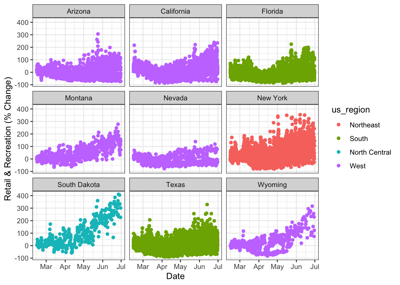
ggplot(early_covid_period_data, aes(dt_date,
                                    parks_percent_change_from_baseline,
                                    color=us_region)) +
  #geom_point() +
  geom_jitter() +
  facet_wrap(.~sub_region_1) +
  labs(x= "Date", y="Retail & Recreation (% Change)") +
  theme_bw(base_size = 16) +
  theme(axis.text.x = element_text(angle=90))
## Warning: Removed 40493 rows containing missing values (geom_point).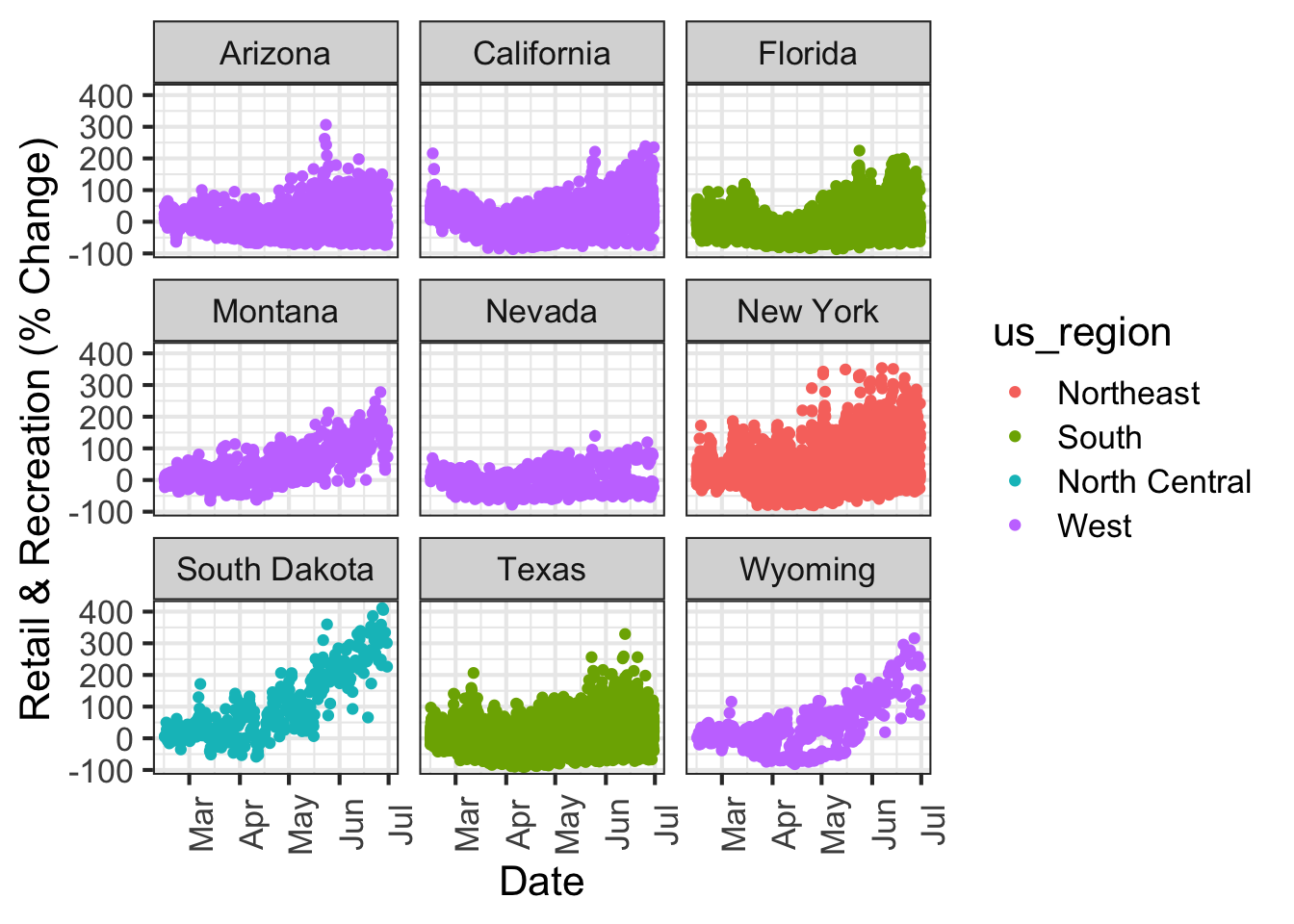
fig1 <- ggplot(early_covid_period_data, aes(dt_date,
                                    retail_and_recreation_percent_change_from_baseline,
                                    color=us_region)) +
  #geom_point() +
  #geom_jitter() +
  geom_smooth() +
  facet_wrap(.~sub_region_1) +
  labs(x= "Date", y="Retail & Recreation (% Change)",
       #color="State",
       tag = "Figure 1",
       title = "Google Mobility: Change over Time",
       subtitle = "i.e., Retail & Recreation, early COVID-19 period (01/20 - 06/20)",
       caption = "Google Mobility: Retail & Recreation (% Change) over early COVID period (01/20 - 06/20)") +
  theme_bw(base_size = 12, base_family = "Arial")

fig2 <- ggplot(early_covid_period_data, aes(dt_date,
                                    parks_percent_change_from_baseline,
                                    color=us_region)) +
  #geom_point() +
  #geom_jitter() +
  geom_smooth() +
  facet_wrap(.~sub_region_1) +
  labs(x= "Date", y="Retail & Recreation (% Change)",
       #color="State",
       tag = "Figure 2",
       title = "Google Mobility: Change over Time",
       subtitle = "i.e., Parks, early COVID-19 period (01/20 - 06/20)",
       caption = "Google Mobility: Parks (% Change) over early COVID period (01/20 - 06/20)") +
  theme_bw(base_size = 12, base_family = "Arial")
fig1
## `geom_smooth()` using method = 'gam' and formula 'y ~ s(x, bs = "cs")'## Warning: Removed 16583 rows containing non-finite values (stat_smooth).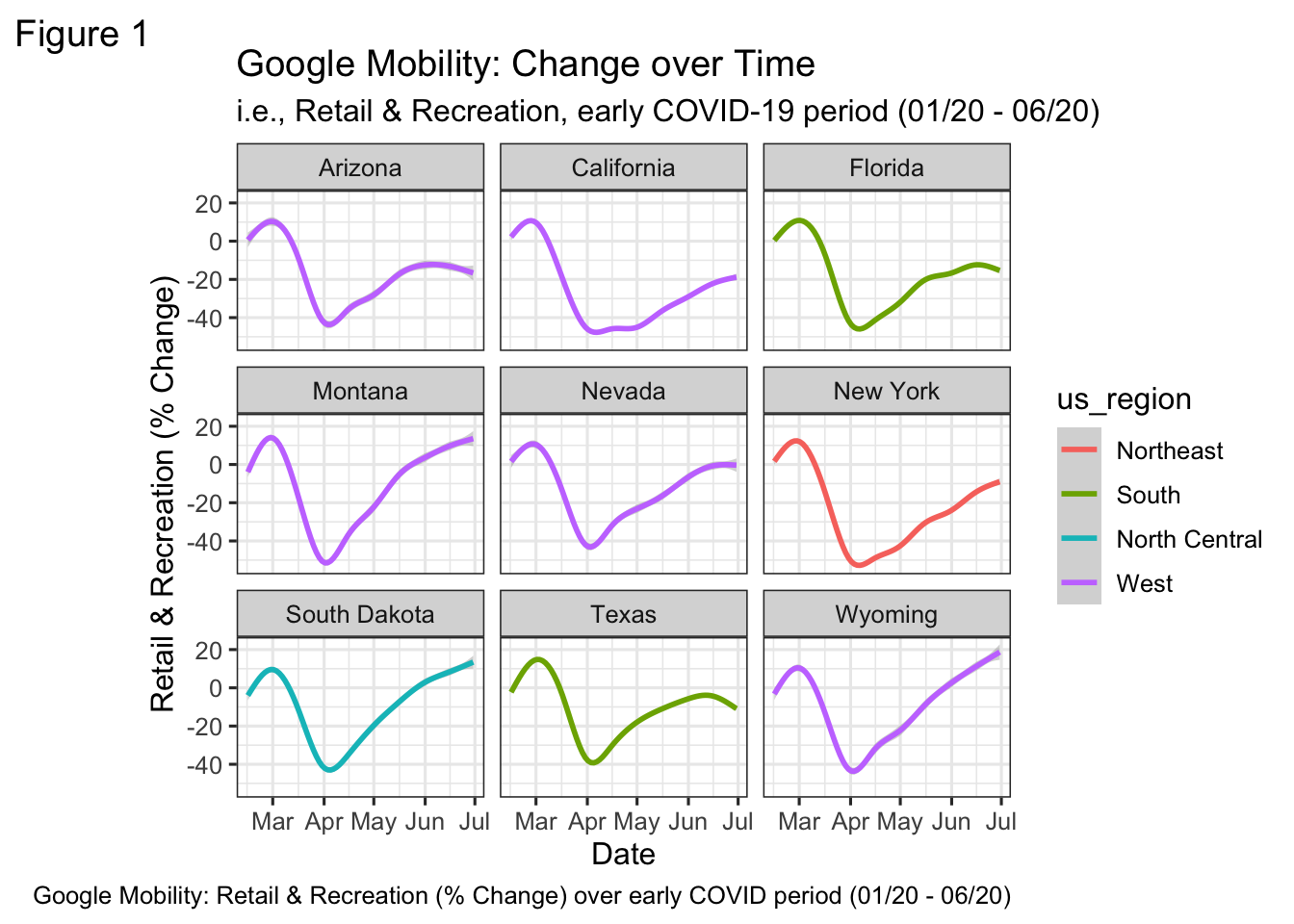
fig2## `geom_smooth()` using method = 'gam' and formula 'y ~ s(x, bs = "cs")'## Warning: Removed 40493 rows containing non-finite values (stat_smooth).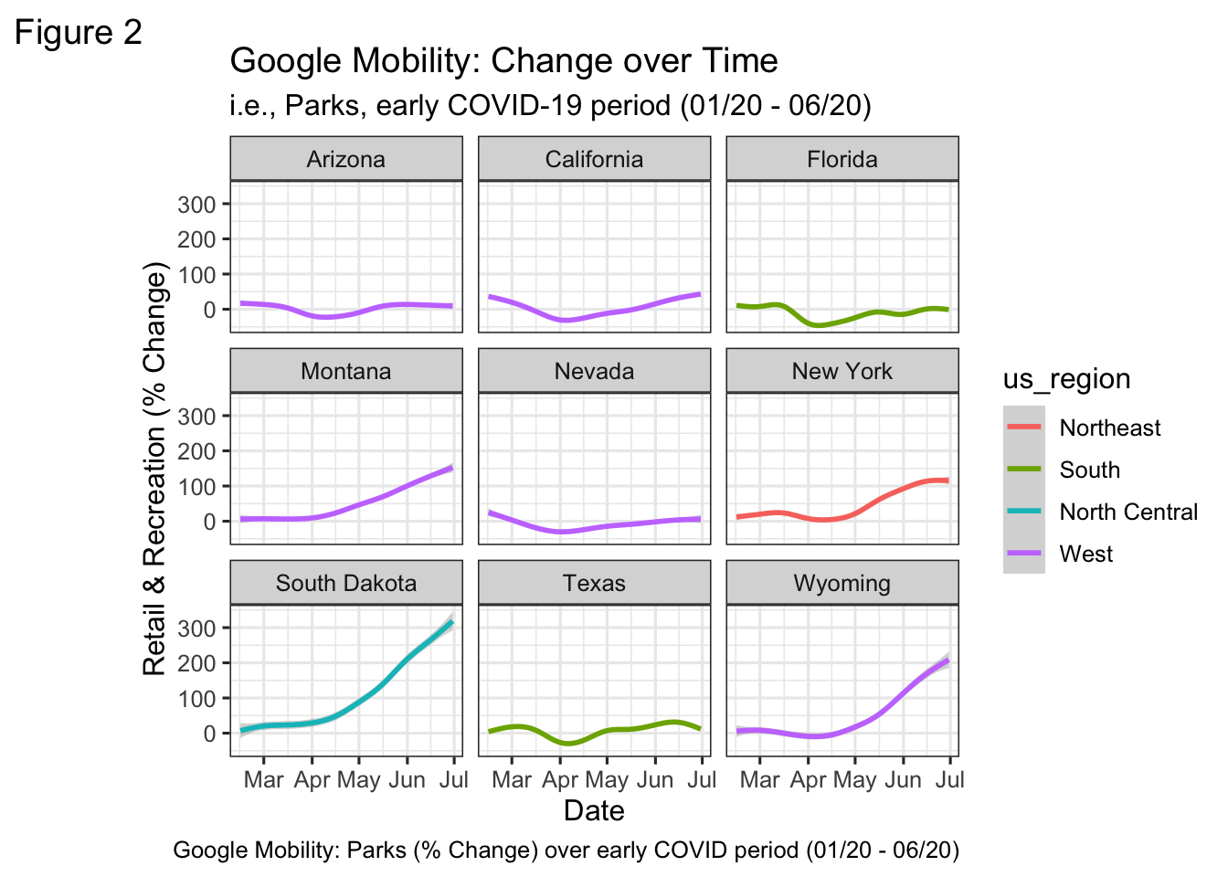
8.16 Evaluate regions of most change
largest_changes_parks_long <- google_mobility_US %>%
  group_by(sub_region_1, dt_year) %>%
  summarise(avg_change_parks = mean(parks_percent_change_from_baseline, na.rm=T)) %>%
  arrange(sub_region_1)
## `summarise()` has grouped output by 'sub_region_1'. You can override using the `.groups`
## argument.
largest_changes_parks_wide <- largest_changes_parks_long %>%
  #pivot_wider(id_cols=c())
  pivot_wider(names_from = dt_year, values_from = avg_change_parks) %>%
  mutate(change_2021_2020 = `2021` - `2020`)

top10_changes <- largest_changes_parks_wide %>%
  arrange(-change_2021_2020) %>%
  head(n=10)

bottom10_changes <- largest_changes_parks_wide %>%
  arrange(change_2021_2020) %>%
  head(n=10)

largest_changes_parks_long
## # A tibble: 156 × 3
## # Groups: sub_region_1 [52]
## sub_region_1 dt_year avg_change_parks
## <chr> <dbl> <dbl>
## 1 Alabama 2020 17.9
## 2 Alabama 2021 7.88
## 3 Alabama 2022 18.0
## 4 Alaska 2020 52.9
## 5 Alaska 2021 59.8
## 6 Alaska 2022 62.5
## 7 Arizona 2020 -1.97
## 8 Arizona 2021 -3.51
## 9 Arizona 2022 -0.316
## 10 Arkansas 2020 48.2
## # … with 146 more rows
largest_changes_parks_wide## # A tibble: 52 × 5
## # Groups: sub_region_1 [52]
## sub_region_1 `2020` `2021` `2022` change_2021_2020
## <chr> <dbl> <dbl> <dbl> <dbl>
## 1 Alabama 17.9 7.88 18.0 -10.0
## 2 Alaska 52.9 59.8 62.5 6.90
## 3 Arizona -1.97 -3.51 -0.316 -1.54
## 4 Arkansas 48.2 44.6 46.8 -3.54
## 5 California 6.17 7.84 8.79 1.67
## 6 Colorado 23.2 14.6 -1.69 -8.60
## 7 Connecticut 51.2 44.6 36.4 -6.62
## 8 Delaware 46.8 52.1 31.5 5.30
## 9 District of Columbia -34.8 -17.1 -14.9 17.7
## 10 Florida -14.7 -8.25 3.72 6.49
## # … with 42 more rows
top10_changes## # A tibble: 10 × 5
## # Groups: sub_region_1 [10]
## sub_region_1 `2020` `2021` `2022` change_2021_2020
## <chr> <dbl> <dbl> <dbl> <dbl>
## 1 Hawaii -46.5 -27.8 -16.8 18.6
## 2 District of Columbia -34.8 -17.1 -14.9 17.7
## 3 Rhode Island 69.2 82.3 65.4 13.1
## 4 South Carolina 23.2 34.7 46.3 11.4
## 5 Maine 59.0 70.0 48.3 10.9
## 6 Vermont 52.8 63.0 60.9 10.2
## 7 Alaska 52.9 59.8 62.5 6.90
## 8 Florida -14.7 -8.25 3.72 6.49
## 9 Tennessee 33.6 39.3 35.6 5.70
## 10 Delaware 46.8 52.1 31.5 5.30
bottom10_changes## # A tibble: 10 × 5
## # Groups: sub_region_1 [10]
## sub_region_1 `2020` `2021` `2022` change_2021_2020
## <chr> <dbl> <dbl> <dbl> <dbl>
## 1 Massachusetts 59.3 44.6 28.5 -14.7
## 2 Utah 61.5 47.6 32.8 -14.0
## 3 Nebraska 64.3 51.0 38.7 -13.3
## 4 Kansas 67.3 54.5 44.9 -12.8
## 5 Mississippi 4.92 -7.07 -6.41 -12.0
## 6 Alabama 17.9 7.88 18.0 -10.0
## 7 West Virginia 3.08 -6.73 -2.22 -9.81
## 8 Ohio 67.7 58.5 38.5 -9.21
## 9 Colorado 23.2 14.6 -1.69 -8.60
## 10 Iowa 63.1 55.1 40.9 -8.00