Ch. 12 Regression, and Multilevel Modeling

12.1 Overview

This example uses data from a reaction time experiment where observers searched for a green circle amongst rectangles, and were asked to report if a line inside the green circle was vertical or horizontal. On some trials, a red rectangle was present, i.e, a distractor. The experiment was conducted in two ways: (1) a random ordering of distractor present and absent trials, and (2) a blocked ordering of distractor present and absent trials. With blocked administration, presumably participants had time to habituate to the distractor and would have a smaller response time decrement as compared with the random presentation condition.

In this example analysis, we will first take a simple approach, and conduct a linear regression, on participant block-level means of response time. Thereafter we will apply multilevel modeling to better capture the nesting and variability inherent in the trial-level data.

12.2 Load libs

12.3 Load data

exp_df <- read_csv("data/exp1.csv")

## Rows: 56896 Columns: 11
## ── Column specification ─────────────────────────────────────────────────────────────────
## Delimiter: ","
## chr (6): practice, datetime, distractor, isRandom, PARTICIPANT, BLOCK
## dbl (5): count_trial_sequence, correct, display_size, response_time, RT
## 
## ℹ Use `spec()` to retrieve the full column specification for this data.
## ℹ Specify the column types or set `show_col_types = FALSE` to quiet this message.

# show data structure
head(exp_df)

## # A tibble: 6 × 11
##   practice count_trial_sequence datetime       correct display_size distractor
##   <chr>                   <dbl> <chr>            <dbl>        <dbl> <chr>     
## 1 yes                         0 11/30/17 15:38       0            5 present   
## 2 yes                         1 11/30/17 15:38       0            5 present   
## 3 yes                         2 11/30/17 15:38       0            5 present   
## 4 yes                         3 11/30/17 15:38       0            5 present   
## 5 yes                         4 11/30/17 15:38       1            5 present   
## 6 yes                         5 11/30/17 15:38       0            5 present   
## # … with 5 more variables: response_time <dbl>, isRandom <chr>,
## #   PARTICIPANT <chr>, RT <dbl>, BLOCK <chr>

12.4 Pre-process data

# filter
exp_pp <- exp_df %>%
  filter(!is.na(PARTICIPANT))

12.4.1 Create additional columns, remove columns

exp_pp_ = exp_pp %>%
  mutate(is_practice = ifelse(practice == "yes", 1, 0)) %>%
  mutate(TRIAL = count_trial_sequence) %>%
  select(-count_trial_sequence, -response_time, -practice) %>%
  select(datetime, PARTICIPANT, BLOCK, TRIAL, is_practice, correct, RT, everything()) %>%
  mutate(EXP_BLOCK_RANDOM = ifelse(isRandom == "blocked", 0, 1))

12.4.2 Get unique metadata

metadata = exp_pp_  %>%
  select(datetime, contains("DT_"), PARTICIPANT, contains("EXP_")) %>%
  distinct()

12.5 Produce simple aggregates

# overall means and record count by participant
part_means = exp_pp_ %>%
  group_by(PARTICIPANT, datetime) %>%
  summarise(mean_rt = mean(RT, na.rm=T),
            sd_rt = sd(RT, na.rm=T),
            q10_rt = quantile(RT, probs=0.1, na.rm=T),
            q90_rt = quantile(RT, probs=0.9, na.rm=T),
            n_correct = sum(correct),
            n = n()) %>%
  inner_join(metadata)

## `summarise()` has grouped output by 'PARTICIPANT'. You can override using the `.groups`
## argument.
## Joining, by = c("PARTICIPANT", "datetime")

# overall means by block
part_means_byblock = exp_pp_ %>%
  group_by(PARTICIPANT, datetime, BLOCK, is_practice, distractor) %>%
  summarise(mean_rt = mean(RT, na.rm=T),
            sd_rt = sd(RT, na.rm=T),
            q10_rt = quantile(RT, probs=0.1, na.rm=T),
            q90_rt = quantile(RT, probs=0.9, na.rm=T),
            n_correct = sum(correct),
            n = n()) %>%
  inner_join(metadata)

## `summarise()` has grouped output by 'PARTICIPANT', 'datetime', 'BLOCK', 'is_practice'.
## You can override using the `.groups` argument.
## Joining, by = c("PARTICIPANT", "datetime")

12.5.1 Mean center the reaction times

exp_m = exp_pp_ %>%
  inner_join(part_means) %>%
  mutate(imean_c_RT = RT - mean_rt)

## Joining, by = c("datetime", "PARTICIPANT", "EXP_BLOCK_RANDOM")

12.6 Data visualization

ggplot(part_means_byblock %>% filter(!is_practice), aes(BLOCK, mean_rt, group=BLOCK, color=as.factor(EXP_BLOCK_RANDOM))) + 
  geom_boxplot() +
  facet_grid(. ~ EXP_BLOCK_RANDOM) +
  theme_bw() +
  labs(x= "Experiment Block", y = "Mean Response Time (ms)")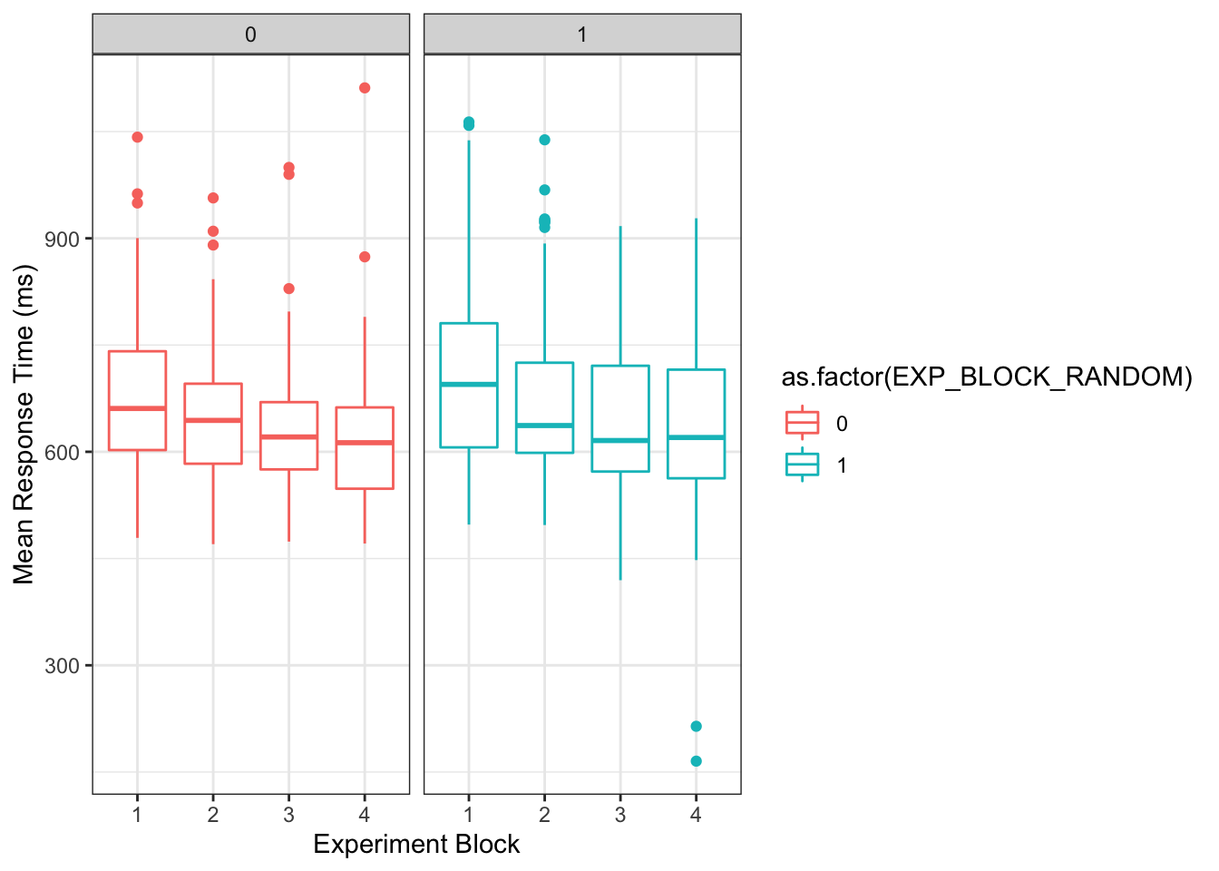

12.7 Predictive Modeling

12.8 Run simple regression on block means

fit = lm(mean_rt ~ n_correct + distractor, data=part_means_byblock)
summary(fit)

## 
## Call:
## lm(formula = mean_rt ~ n_correct + distractor, data = part_means_byblock)
## 
## Residuals:
##     Min      1Q  Median      3Q     Max 
## -617.82 -127.71  -35.44   84.02 1053.19 
## 
## Coefficients:
##                   Estimate Std. Error t value Pr(>|t|)    
## (Intercept)       784.1357     9.3788  83.608   <2e-16 ***
## n_correct          -1.9625     0.1634 -12.011   <2e-16 ***
## distractorpresent  20.9713    10.5291   1.992   0.0466 *  
## ---
## Signif. codes:  0 '***' 0.001 '**' 0.01 '*' 0.05 '.' 0.1 ' ' 1
## 
## Residual standard error: 205.8 on 1525 degrees of freedom
## Multiple R-squared:  0.08874,    Adjusted R-squared:  0.08754 
## F-statistic: 74.25 on 2 and 1525 DF,  p-value: < 2.2e-16

12.8.1 Show resulting model equation

# show model equation
library(equatiomatic)
extract_eq(fit, use_coefs=TRUE, wrap=TRUE)

\[ \begin{aligned} \operatorname{\widehat{mean\_rt}} &= 784.14 - 1.96(\operatorname{n\_correct}) + 20.97(\operatorname{distractor}_{\operatorname{present}}) \end{aligned} \]

12.9 Run as series of incremental multilevel model

# run models, starting with unconditional means model
fitm_0  = lme4::lmer(RT ~ 1 + (1|PARTICIPANT),
                      data=exp_pp_)
fitm_1  = lme4::lmer(RT ~ TRIAL + (1|PARTICIPANT),
                      data=exp_pp_)
fitm_2  = lme4::lmer(RT ~ TRIAL + is_practice + (1|PARTICIPANT),
                      data=exp_pp_)
fitm_3  = lme4::lmer(RT ~ TRIAL + is_practice + correct + (1|PARTICIPANT),
                      data=exp_pp_)
fitm_4  = lme4::lmer(RT ~ TRIAL + is_practice + correct +
                       distractor + 
                       (1|PARTICIPANT),
                      data=exp_pp_)
fitm_5  = lme4::lmer(RT ~ TRIAL + is_practice + correct +
                       distractor + 
                       display_size + 
                       EXP_BLOCK_RANDOM +
                       (1|PARTICIPANT),
                      data=exp_pp_)

extract_eq(fitm_5, use_coefs=TRUE, wrap=TRUE)

\[ \begin{aligned} \operatorname{\widehat{RT}}_{i} &\sim N \left(\mu, \sigma^2 \right) \\ \mu &=796.63_{\alpha_{j[i]}} - 0.29_{\beta_{1}}(\operatorname{TRIAL}) + 111.09_{\beta_{2}}(\operatorname{is\_practice}) - 98.78_{\beta_{3}}(\operatorname{correct})\ + \\ &\quad 20.84_{\beta_{4}}(\operatorname{distractor}_{\operatorname{present}}) + 1.53_{\beta_{5}}(\operatorname{display\_size}) - 6.5_{\beta_{6}}(\operatorname{EXP\_BLOCK\_RANDOM}) \\ \alpha_{j} &\sim N \left(0, 98.99 \right) \text{, for PARTICIPANT j = 1,} \dots \text{,J} \end{aligned} \]

12.9.1 Compare models

# compare models
anova(fitm_0, fitm_1, fitm_2, fitm_3, fitm_4, fitm_5)

## refitting model(s) with ML (instead of REML)

## Data: exp_pp_
## Models:
## fitm_0: RT ~ 1 + (1 | PARTICIPANT)
## fitm_1: RT ~ TRIAL + (1 | PARTICIPANT)
## fitm_2: RT ~ TRIAL + is_practice + (1 | PARTICIPANT)
## fitm_3: RT ~ TRIAL + is_practice + correct + (1 | PARTICIPANT)
## fitm_4: RT ~ TRIAL + is_practice + correct + distractor + (1 | PARTICIPANT)
## fitm_5: RT ~ TRIAL + is_practice + correct + distractor + display_size + EXP_BLOCK_RANDOM + (1 | PARTICIPANT)
##        npar    AIC    BIC  logLik deviance    Chisq Df Pr(>Chisq)    
## fitm_0    3 775163 775190 -387579   775157                           
## fitm_1    4 772908 772944 -386450   772900 2256.615  1  < 2.2e-16 ***
## fitm_2    5 771229 771274 -385610   771219 1681.167  1  < 2.2e-16 ***
## fitm_3    6 770470 770523 -385229   770458  761.500  1  < 2.2e-16 ***
## fitm_4    7 770331 770394 -385159   770317  140.332  1  < 2.2e-16 ***
## fitm_5    9 770323 770404 -385152   770305   12.428  2   0.002001 ** 
## ---
## Signif. codes:  0 '***' 0.001 '**' 0.01 '*' 0.05 '.' 0.1 ' ' 1

12.10 Create publication-ready table of results

sjPlot::tab_model(fitm_0, fitm_5)

	RT			RT
Predictors	Estimates	CI	p	Estimates	CI	p
(Intercept)	670.44	653.24 – 687.63	<0.001	796.63	774.02 – 819.25	<0.001
TRIAL				-0.29	-0.30 – -0.27	<0.001
is practice				111.09	105.44 – 116.74	<0.001
correct				-98.78	-105.82 – -91.73	<0.001
distractor [present]				20.84	17.40 – 24.29	<0.001
display size				1.53	0.67 – 2.39	0.001
EXP BLOCK RANDOM				-6.50	-28.08 – 15.07	0.555
Random Effects
σ²	47870.23			43951.44
τ₀₀	9588.24 _PARTICIPANT			9799.13 _PARTICIPANT
ICC	0.17			0.18
N	126 _PARTICIPANT			126 _PARTICIPANT
Observations	56896			56896
Marginal R² / Conditional R²	0.000 / 0.167			0.068 / 0.238

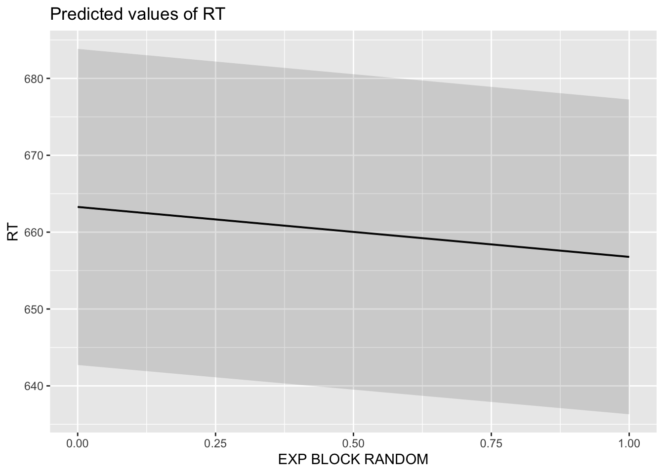
12.11 Create publication-ready figure of results

sjPlot::plot_model(fitm_5, type="pred")

## $TRIAL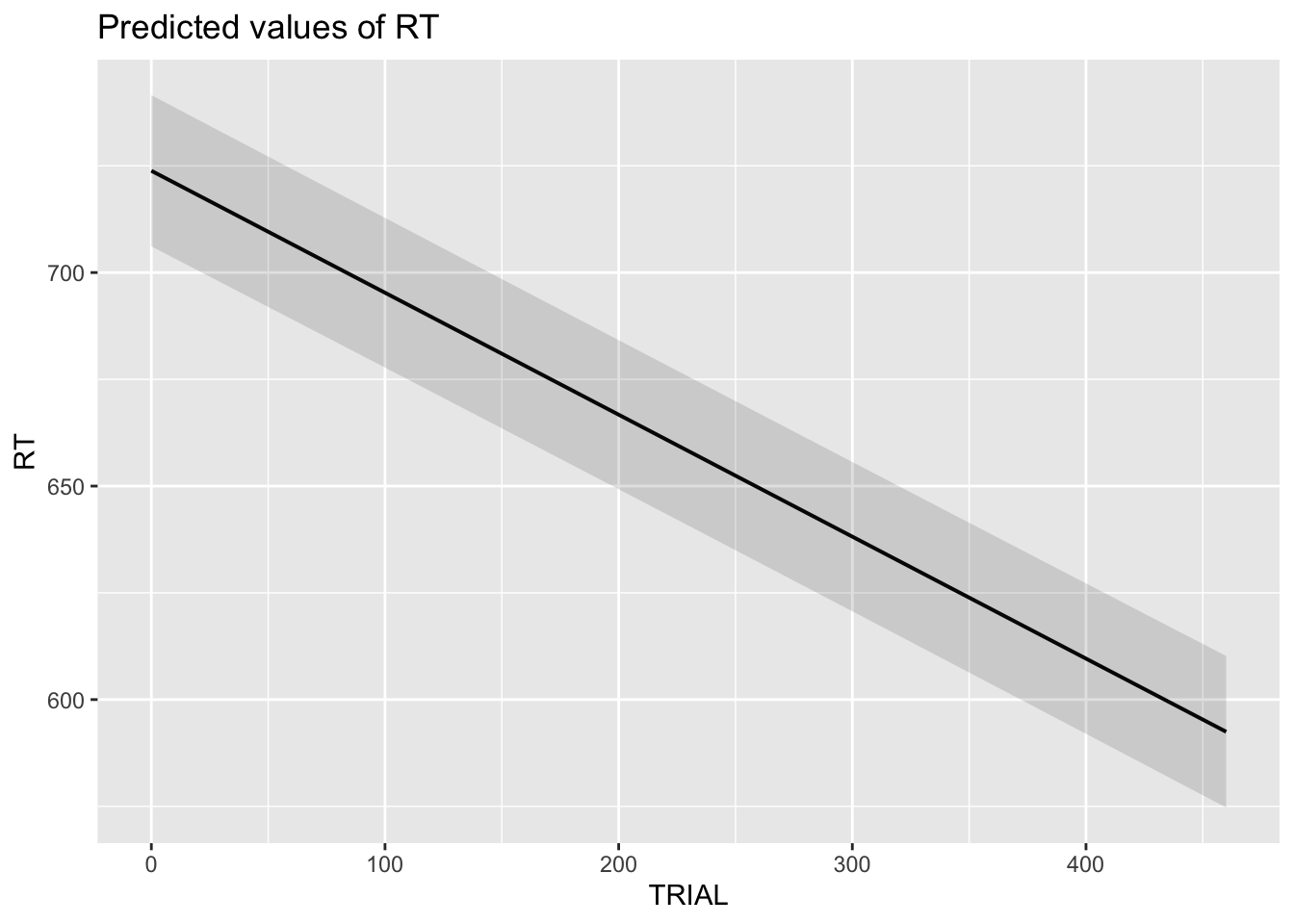

## 
## $is_practice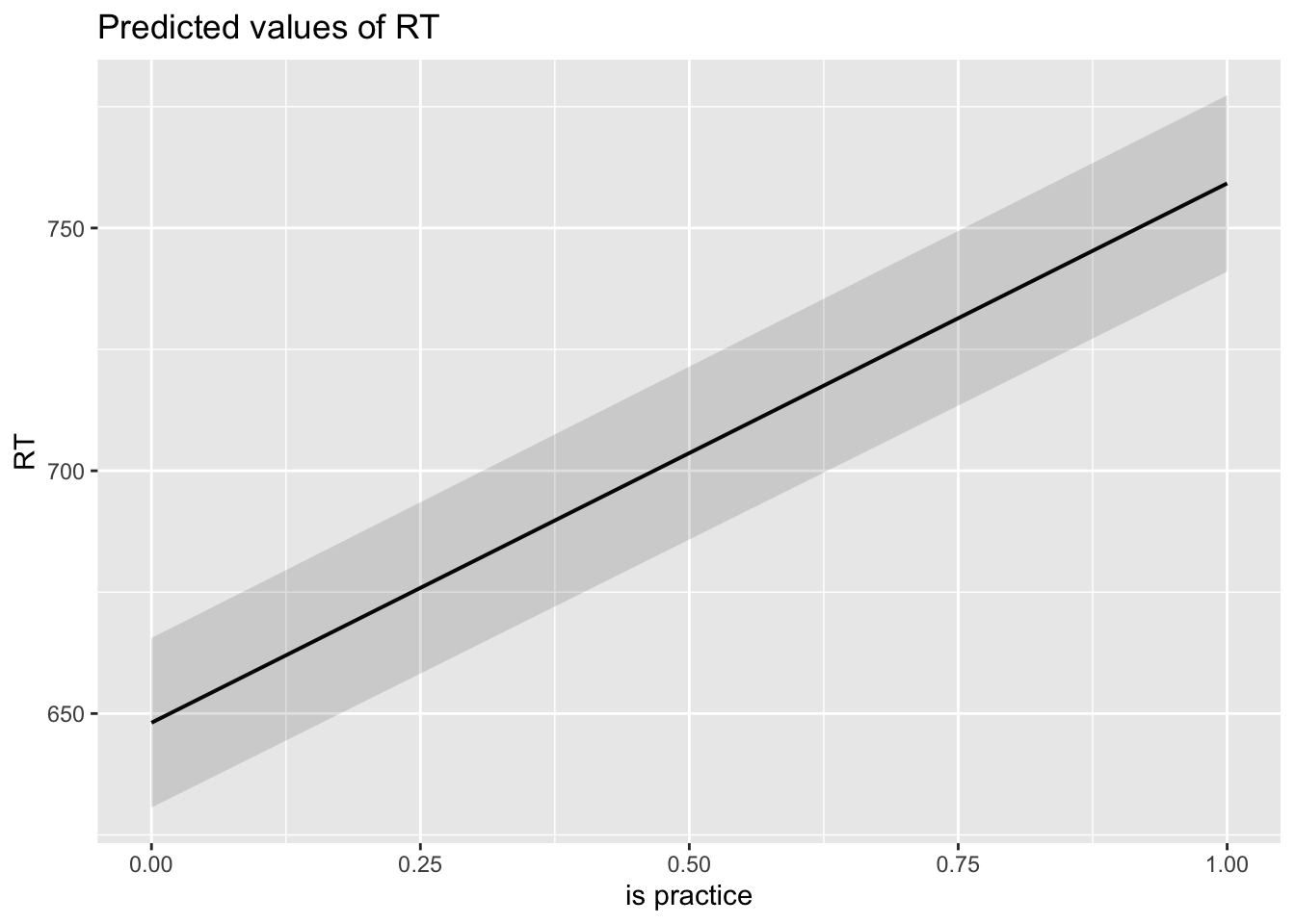

## 
## $correct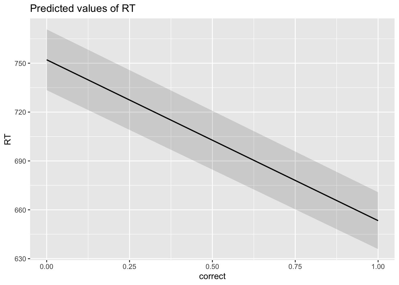

## 
## $distractor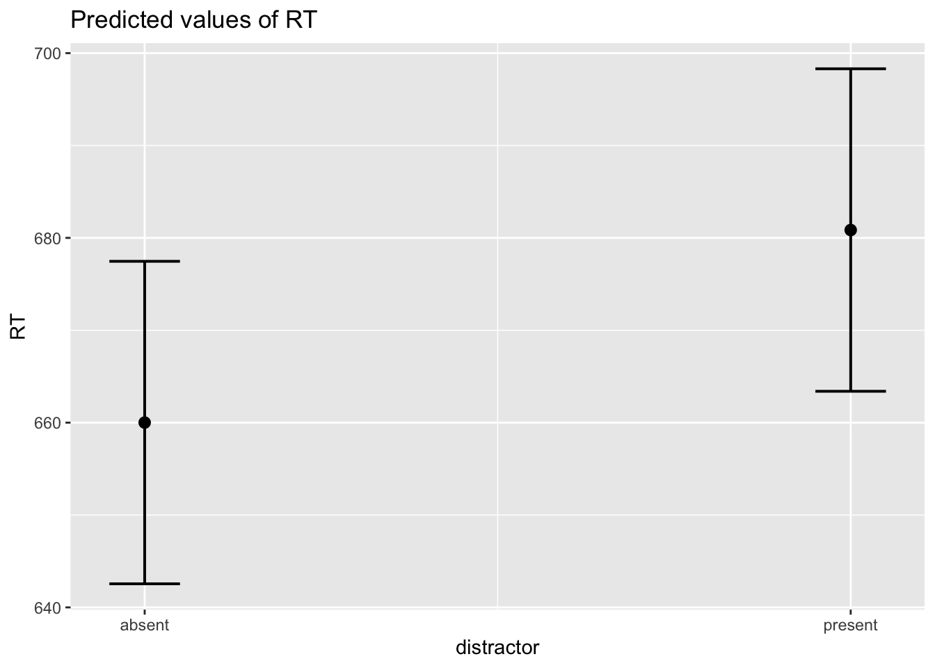

## 
## $display_size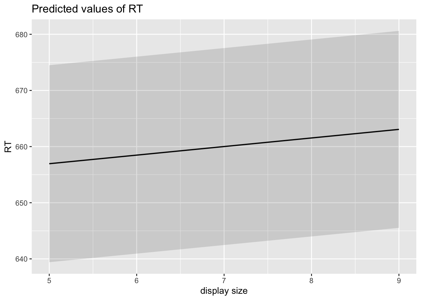

## 
## $EXP_BLOCK_RANDOM

11 Working with APIs

13 Resources