Ch. 9 Working with Text Data

9.1 Background

Text Mining is the process of analyzing text data for key topics, trends, and hidden relationships. Methods include: - Word frequency analysis - Wordclouds - Topic modeling

This collection of methods is especially important since, 80% of the world’s data is in an unstructured format.

9.2 The Secret is Pre-processing

Always consider the data processing implications of your data source. Depending on if you are working with transcriptions form audio or video, or digitized free-entry text, you will want to pre-process your data for misspellings and incorrect transcriptions before proceeding with any text mining.

9.3 Overview

For this example, we will work with product review data from the following open science resource: https://osf.io/tyue9

Salminen, J., Kandpal, C., Kamel, A. M., Jung, S., & Jansen, B. J. (2022). Creating and detecting fake reviews of online products. Journal of Retailing and Consumer Services, 64, 102771. https://doi.org/10.1016/j.jretconser.2021.102771

9.4 Load Libs

library(readr)
library(tidyverse)
library(tidytext)
library(textdata)
library(topicmodels)
library(wordcloud)

## Loading required package: RColorBrewer

library(ggwordcloud)

9.5 Load full dataset

# %%%%%%%%%%%%%%%%%%%%%%%%%%%%%%%%%%%%%%%%%%%%%%%%%%%%%%%%%%%%%%%%%%%%%%%%%%%%%

df <- readr::read_csv("data/fake reviews dataset.csv") %>%
  mutate(id = row_number()) %>% # add row id
  select(id, category, everything()) %>%
  mutate(text_clean = stringr::str_replace_all(text_, "[^[:alnum:]]", " "))

## Rows: 40432 Columns: 4
## ── Column specification ─────────────────────────────────────────────────────────────────
## Delimiter: ","
## chr (3): category, label, text_
## dbl (1): rating
## 
## ℹ Use `spec()` to retrieve the full column specification for this data.
## ℹ Specify the column types or set `show_col_types = FALSE` to quiet this message.

  # clean up text a bit


unique(df$category)

##  [1] "Home_and_Kitchen_5"           "Sports_and_Outdoors_5"       
##  [3] "Electronics_5"                "Movies_and_TV_5"             
##  [5] "Tools_and_Home_Improvement_5" "Pet_Supplies_5"              
##  [7] "Kindle_Store_5"               "Books_5"                     
##  [9] "Toys_and_Games_5"             "Clothing_Shoes_and_Jewelry_5"

unique(df$label)

## [1] "CG" "OR"

9.6 Produce a data quality report

df_dq <- skimr::skim(df)

knitr::kable(df_dq)# %>% kableExtra::kable_minimal(.)

skim_type	skim_variable	complete_rate	character.min	character.max	character.empty	character.n_unique	character.whitespace	numeric.mean	numeric.sd	numeric.p0	numeric.p25	numeric.p50	numeric.p75	numeric.p100	numeric.hist
character	category	1	7	28	0	10	0	NA	NA	NA	NA	NA	NA	NA	NA
character	label	1	2	2	0	2	0	NA	NA	NA	NA	NA	NA	NA	NA
character	text_	1	5	2827	0	40411	0	NA	NA	NA	NA	NA	NA	NA	NA
character	text_clean	1	5	2827	0	40411	1	NA	NA	NA	NA	NA	NA	NA	NA
numeric	id	1	NA	NA	NA	NA	NA	20216.500000	11671.857379	1	10108.75	20216.5	30324.25	40432	▇▇▇▇▇
numeric	rating	1	NA	NA	NA	NA	NA	4.256579	1.144354	1	4.00	5.0	5.00	5	▁▁▁▂▇

9.7 Not all lexicons are equal

Get proportion of stop_words by lexicon (onix, SMART, snowball). Full listing of words available here.

prop.table(table(stop_words$lexicon))

## 
##      onix     SMART  snowball 
## 0.3516101 0.4969539 0.1514360

If a word you cared about is in the stop word dictionary you will lose it in your analysis. Use the code below if you need to exclude words from the stopword dictionary.

stop_words_filt = stop_words %>%
   filter(word != "better")

# Otherwise continue
stop_words_filt = stop_words

9.8 Tokenize the text

# text mining analyses ----
section_freeresponse_tokens = df %>%
  unnest_tokens(bigram,
                "text_clean",
                token = "ngrams",
                n = 2,
                drop = F) %>%
  separate(bigram, c("word1", "word2"), sep = " ", remove=F) %>%
  filter(!word1 %in% stop_words_filt$word) %>%
  filter(!word2 %in% stop_words_filt$word)

9.9 Compute td-idf statistic

tf_idf = statistic intended to reflect how important word is to a document

# %%%%%%%%%%%%%%%%%%%%%%%%%%%%%%%%%%%%%%%%%%%%%%%%%%%%%%%%%%%%%%%%%%%%%%%%%%%%%

section_fr_1_tf_idf = section_freeresponse_tokens %>%
  count(category, word1) %>%
  bind_tf_idf(word1, category, n) %>%
  arrange(desc(tf_idf))

knitr::kable(head(section_fr_1_tf_idf))# %>% kableExtra::kable_paper(.)

category	word1	n	tf	idf	tf_idf
Pet_Supplies_5	litter	268	0.0127032	1.2039728	0.0152943
Kindle_Store_5	author	333	0.0115277	1.2039728	0.0138790
Pet_Supplies_5	dogs	415	0.0196710	0.6931472	0.0136349
Toys_and_Games_5	leapfrog	104	0.0054582	2.3025851	0.0125679
Tools_and_Home_Improvement_5	bosch	211	0.0092224	1.2039728	0.0111036
Toys_and_Games_5	lego	91	0.0047759	2.3025851	0.0109969

section_fr_2_tf_idf = section_freeresponse_tokens %>%
  count(label, word1) %>%
  bind_tf_idf(word1, label, n) %>%
  arrange(desc(tf_idf))

knitr::kable(head(section_fr_2_tf_idf))# %>% kableExtra::kable_paper(.)

label	word1	n	tf	idf	tf_idf
CG	treme	24	0.0003563	0.6931472	0.0002470
CG	mcclone	22	0.0003266	0.6931472	0.0002264
OR	anti	52	0.0003135	0.6931472	0.0002173
CG	galt	21	0.0003117	0.6931472	0.0002161
CG	60lb	20	0.0002969	0.6931472	0.0002058
CG	rosanna	20	0.0002969	0.6931472	0.0002058

# vis tf_idf ----
section_fr_1_tf_idf %>%
  group_by(category) %>%
  slice_max(tf_idf, n = 3) %>%
  ungroup() %>%
  ggplot(aes(tf_idf, fct_reorder(word1, tf_idf), fill = category)) +
  geom_col(show.legend = FALSE) +
  facet_wrap(~category, ncol = 2, scales = "free") +
  labs(x = "tf-idf", y = NULL)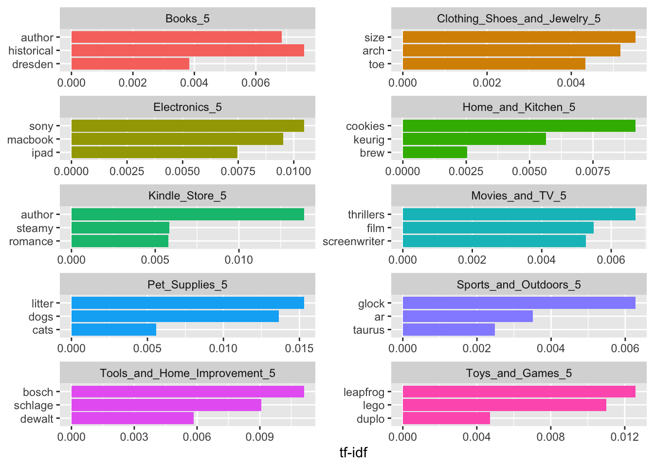

section_fr_2_tf_idf %>%
  group_by(label) %>%
  slice_max(tf_idf, n = 3) %>%
  ungroup() %>%
  ggplot(aes(tf_idf, fct_reorder(word1, tf_idf), fill = label)) +
  geom_col(show.legend = FALSE) +
  facet_wrap(~label, ncol = 2, scales = "free") +
  labs(x = "tf-idf", y = NULL)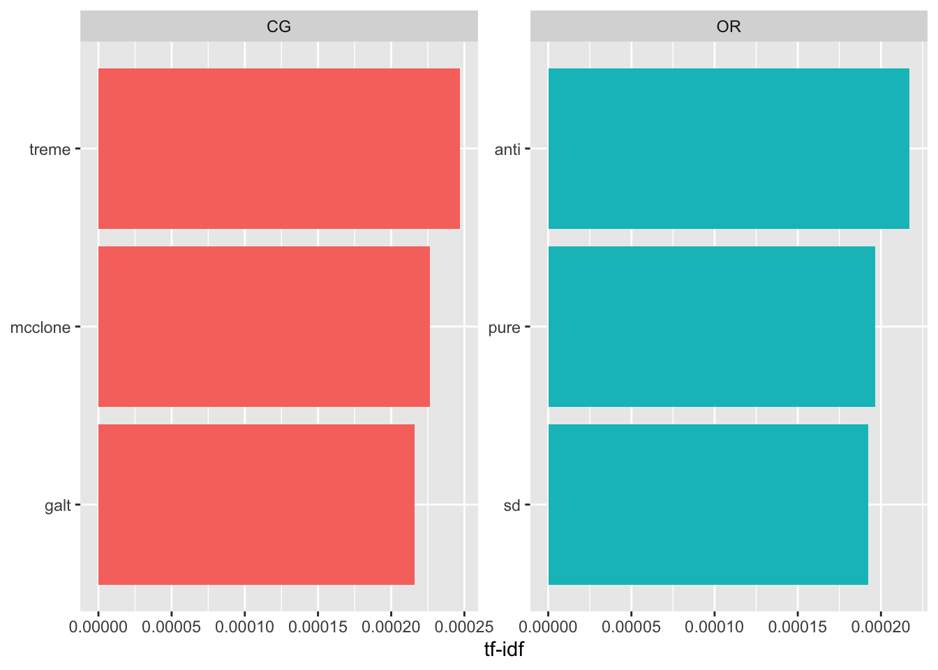

9.10 Generate a wordcloud

# https://towardsdatascience.com/create-a-word-cloud-with-r-bde3e7422e8a
wordcloud::wordcloud(words = section_fr_1_tf_idf %>% pull(word1),
                     freq = section_fr_1_tf_idf %>% pull(n),
                     min.freq = 300,
                     max.words=200,
                     random.order=FALSE,
                     rot.per=0.1)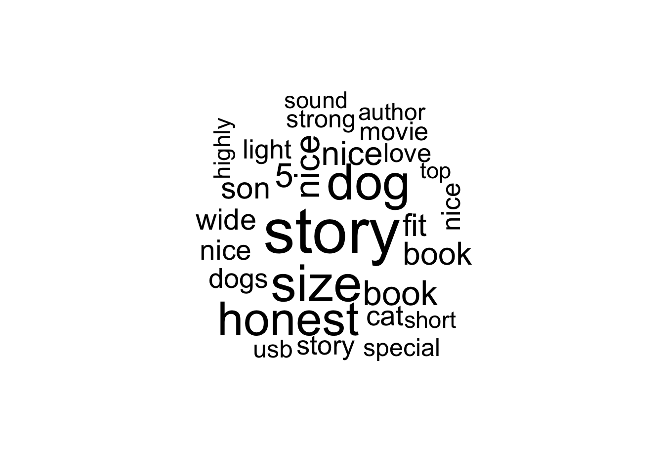

9.11 Conduct simple sentiment analysis

nrc. binary “yes”/“no” for categories positive, negative, anger, anticipation, disgust, fear, joy, sadness, surprise, and trust.
bing. “positive”/“negative” classification.
AFINN. score between -5 (most negative) and 5 (most positive).
loughran. “positive”/“negative”/“litigious”/“uncertainty”/“constraining”/“superflous” classification.

9.11.1 Visualize sentiment distribution in each lexicon

Source code


x1 <- get_sentiments(lexicon = "nrc") %>%
  count(sentiment) %>%
  mutate(lexicon = "nrc")
x2 <- get_sentiments(lexicon = "bing") %>%
  count(sentiment) %>%
  mutate(lexicon = "bing")
x3 <- get_sentiments(lexicon = "afinn") %>%
  count(value) %>%
  mutate(lexicon = "afinn") %>%
  mutate(sentiment = as.character(value)) %>%
  select(-value)
# x4 <- get_sentiments(lexicon = "loughran") %>%
#   count(sentiment) %>%
#   mutate(lexicon = "loughran")
x <- bind_rows(x1, x2, x3)

ggplot(x, aes(x = fct_reorder(sentiment, n), y = n, fill = lexicon)) +
  geom_col(show.legend = FALSE) +
  coord_flip() +
  labs(title = "Sentiment Counts", x = "", y = "") +
  facet_wrap(~ lexicon, scales = "free")


# %%%%%%%%%%%%%%%%%%%%%%%%%%%%%%%%%%%%%%%%%%%%%%%%%%%%%%%%%%%%%%%%%%%%%%%%%%%%%

# sentiment analysis ----
AFINN <- get_sentiments("afinn")

# more options ---
# get_sentiments(lexicon = c("bing", "afinn", "loughran", "nrc"))

# %%%%%%%%%%%%%%%%%%%%%%%%%%%%%%%%%%%%%%%%%%%%%%%%%%%%%%%%%%%%%%%%%%%%%%%%%%%%%

# merge sentiment with dataset ----
sent_words <- section_freeresponse_tokens %>%
  inner_join(AFINN, by = c(word1 = "word"))

sent_words_fj <- section_freeresponse_tokens %>%
  full_join(AFINN, by = c(word1 = "word"))

# produce various aggregates of sentiment ----
count_words_by_sent = sent_words %>%
  count(category, value, sort = TRUE) %>%
  mutate(n_cut = cut(n, c(0,500,3000,Inf)))

9.12 Visualize sentiment

ggplot(count_words_by_sent, aes(value, n_cut)) +
  geom_tile() +
  facet_grid(.~category)

avg_sent_by_category = sent_words %>%
 group_by(category) %>%
  summarise(avg_sent = mean(value, na.rm=T),
            sd_sent = sd(value, na.rm=T))

mv = ggplot(avg_sent_by_category, aes(category, avg_sent)) +
  geom_bar(stat="identity") +
  theme(axis.text.x = element_text(angle=90))

sv = ggplot(avg_sent_by_category, aes(category, sd_sent)) +
  geom_bar(stat="identity") +
  theme(axis.text.x = element_text(angle=90))

cowplot::plot_grid(mv, sv, ncol=2)

9.13 Topic modeling analysis

Coming soon! Resource: https://www.tidytextmining.com/topicmodeling.html

ap_data = section_fr_1_tf_idf %>%
  mutate(word1_ = as.character(word1)) %>%
  cast_dtm(category, word1_, n)

Topic models in practice use larger k values - k=2 works for this example.

ap_lda <- LDA(ap_data, k = 2, control = list(seed = 1234))
ap_topics <- tidy(ap_lda, matrix = "beta")
ap_documents <- tidy(ap_lda, matrix = "gamma")

9.14 Visualize topic modeling results

ap_top_terms <- ap_topics %>%
  filter(!is.na(term)) %>%
  group_by(topic) %>%
  slice_max(beta, n = 20) %>%
  ungroup() %>%
  arrange(topic, -beta)

ap_top_terms %>%
  mutate(term = reorder_within(term, beta, topic)) %>%
  ggplot(aes(beta, term, fill = factor(topic))) +
  geom_col(show.legend = FALSE) +
  facet_wrap(~ topic, scales = "free") +
  scale_y_reordered()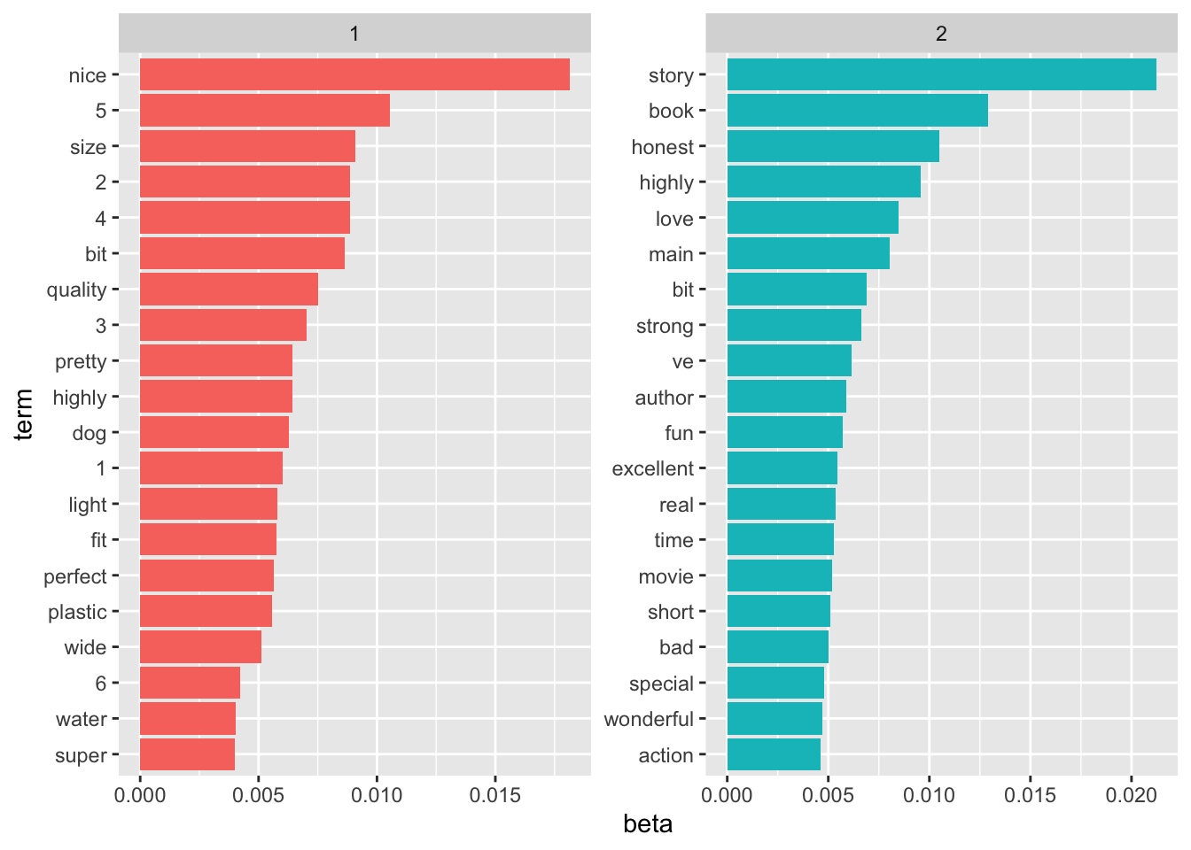

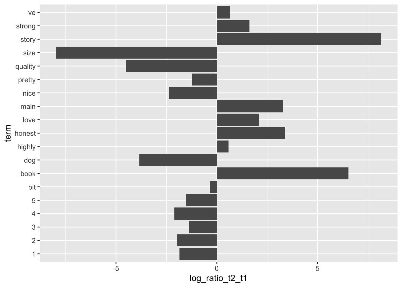
Visualize the terms that had the greatest difference in β between topic 1 and topic 2

threshold = .006 # low values return more words
beta_wide <- ap_topics %>%
  mutate(topic = paste0("topic", topic)) %>%
  pivot_wider(names_from = topic, values_from = beta) %>%
  filter(topic1 > threshold | topic2 > threshold) %>%
  mutate(log_ratio_t2_t1 = log2(topic2 / topic1))

ggplot(beta_wide, aes(log_ratio_t2_t1, term)) +
  geom_bar(stat="identity")

8 Data Wrangling and Visualization of Big Data

10 Working with JSON data